Missing Data

This guide briefly outlines handling missing data in your data set. This is not meant to be a comprehensive treatment of how to deal with missing data. One can teach a whole class or write a whole book on this subject. Instead, the guide provides a brief overview, with some direction on the available R functions that handle missing data.

Bringing data into R

First, let’s load in the required packages for this guide. Depending on when you read this guide, you may need to install some of these packages before calling library().

library(sf)
library(sp)
library(spdep)
library(tidyverse)
library(tmap)

We’ll be using the shapefile saccity.shp. The file contains Sacramento City census tracts with the percent of the tract population living in subsidized housing, which was taken from the U.S. Department of Housing and Urban Development data portal.

We’ll need to read in the shapefile. First, set your working directory to a folder you want to save your data in.

setwd("path to the folder containing saccity.shp")

I saved the file in Github as a zip file. Download that zip file using the function download.file(), unzip it using the function unzip(), and read the file into R using st_read()

download.file(url = "https://raw.githubusercontent.com/crd230/data/master/saccity.zip", destfile = "saccity.zip")
unzip(zipfile = "saccity.zip")
sac.city.tracts.sf <- st_read("saccity.shp")

## Reading layer `saccity' from data source `/Users/noli/Documents/UCD/teaching/CRD 230/Lab/crd230.github.io/saccity.shp' using driver `ESRI Shapefile'
## Simple feature collection with 120 features and 3 fields
## geometry type:  MULTIPOLYGON
## dimension:      XY
## bbox:           xmin: -121.5601 ymin: 38.43757 xmax: -121.3627 ymax: 38.6856
## epsg (SRID):    4269
## proj4string:    +proj=longlat +datum=NAD83 +no_defs

In case you are having problems with the above code, try installing the package utils. If you are still having problems, download the zip file from Canvas (Additional data). Save that file into the folder you set your working directory to. Then use st_read() as above.

Let’s look at the tibble.

sac.city.tracts.sf

## Simple feature collection with 120 features and 3 fields
## geometry type:  MULTIPOLYGON
## dimension:      XY
## bbox:           xmin: -121.5601 ymin: 38.43757 xmax: -121.3627 ymax: 38.6856
## epsg (SRID):    4269
## proj4string:    +proj=longlat +datum=NAD83 +no_defs
## First 10 features:
##          GEOID                                              NAME psubhous
## 1  06067000100     Census Tract 1, Sacramento County, California       NA
## 2  06067000200     Census Tract 2, Sacramento County, California       NA
## 3  06067000300     Census Tract 3, Sacramento County, California       NA
## 4  06067000400     Census Tract 4, Sacramento County, California     2.18
## 5  06067000500     Census Tract 5, Sacramento County, California     7.89
## 6  06067000600     Census Tract 6, Sacramento County, California    15.44
## 7  06067000700     Census Tract 7, Sacramento County, California    17.00
## 8  06067000800     Census Tract 8, Sacramento County, California     9.17
## 9  06067001101 Census Tract 11.01, Sacramento County, California     5.24
## 10 06067001200    Census Tract 12, Sacramento County, California    10.05
##                          geometry
## 1  MULTIPOLYGON (((-121.4472 3...
## 2  MULTIPOLYGON (((-121.4505 3...
## 3  MULTIPOLYGON (((-121.4615 3...
## 4  MULTIPOLYGON (((-121.4748 3...
## 5  MULTIPOLYGON (((-121.487 38...
## 6  MULTIPOLYGON (((-121.487 38...
## 7  MULTIPOLYGON (((-121.5063 3...
## 8  MULTIPOLYGON (((-121.5116 3...
## 9  MULTIPOLYGON (((-121.4989 3...
## 10 MULTIPOLYGON (((-121.48 38....

And make sure it looks like Sacramento city

tm_shape(sac.city.tracts.sf) +
  tm_polygons()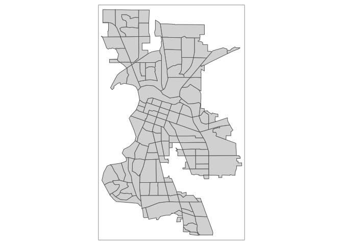

Cool? Cool.

Summarizing data with missing values

The variable psubhous gives us the percent of the tract population living in subsidized housing. What is the mean of this variable?

sac.city.tracts.sf %>% summarize(mean = mean(psubhous))

## Simple feature collection with 1 feature and 1 field
## geometry type:  POLYGON
## dimension:      XY
## bbox:           xmin: -121.5601 ymin: 38.43757 xmax: -121.3627 ymax: 38.6856
## epsg (SRID):    4269
## proj4string:    +proj=longlat +datum=NAD83 +no_defs
##   mean                       geometry
## 1   NA POLYGON ((-121.409 38.50368...

We get “NA” which tells us that there are some neighborhoods with missing data. If a variable has an NA, most R functions summarizing that variable automatically yield an NA.

What if we try to do some kind of spatial data analysis on the data? Surely, R won’t give us a problem since spatial is special, right? Let’s calculate the Moran’s I (see Lab 5) for psubhous.

#Turn sac.city.tracts.sf into an sp object.
sac.city.tracts.sp <- as(sac.city.tracts.sf, "Spatial")

sacb<-poly2nb(sac.city.tracts.sp, queen=T)
sacw<-nb2listw(sacb, style="W")
moran.test(sac.city.tracts.sp$psubhous, sacw)

## Error in na.fail.default(x): missing values in object

Similar to nonspatial data functions, R will force you to deal with your missing data values. In this case, R gives us an error.

Summarizing the extent of missingness

Before you do any analysis on your data, it’s a good idea to check the extent of missingness in your data set. The best way to do this is to use the function aggr(), which is a part of the VIM package. Install this package and load it into R.

install.packages("VIM")
library(VIM)

Then run the aggr() function as follows

summary(aggr(sac.city.tracts.sf))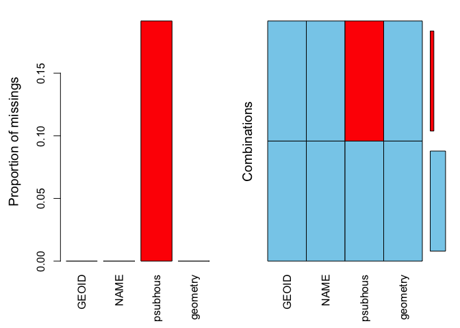

## 
##  Missings per variable: 
##  Variable Count
##     GEOID     0
##      NAME     0
##  psubhous    23
##  geometry     0
## 
##  Missings in combinations of variables: 
##  Combinations Count  Percent
##       0:0:0:0    97 80.83333
##       0:0:1:0    23 19.16667

The results show two tables and two plots. The left-hand side plot shows the proportion of cases that are missing values for each variable in the data set. The right-hand side plot shows which combinations of variables are missing. The first table shows the number of cases that are missing values for each variable in the data set. The second table shows the percent of cases missing values based on combinations of variables. The results show that 23 or 19% of census tracts are missing values on the variable psubhous.

Exclude missing data

The most simplest way for dealing with cases having missing values is to delete them. You do this using the filter() command

sac.city.tracts.sf.rm <- filter(sac.city.tracts.sf, is.na(psubhous) != TRUE)

You now get your mean

sac.city.tracts.sf.rm %>% summarize(mean = mean(psubhous))

## Simple feature collection with 1 feature and 1 field
## geometry type:  POLYGON
## dimension:      XY
## bbox:           xmin: -121.5601 ymin: 38.43757 xmax: -121.3627 ymax: 38.68522
## epsg (SRID):    4269
## proj4string:    +proj=longlat +datum=NAD83 +no_defs
##      mean                       geometry
## 1 6.13866 POLYGON ((-121.409 38.50368...

And your Moran’s I

#Turn sac.city.tracts.sf into an sp object.
sac.city.tracts.sp.rm <- as(sac.city.tracts.sf.rm, "Spatial")

sacb.rm<-poly2nb(sac.city.tracts.sp.rm, queen=T)
sacw.rm<-nb2listw(sacb.rm, style="W")
moran.test(sac.city.tracts.sp.rm$psubhous, sacw.rm)

## 
##  Moran I test under randomisation
## 
## data:  sac.city.tracts.sp.rm$psubhous  
## weights: sacw.rm    
## 
## Moran I statistic standard deviate = 1.5787, p-value = 0.0572
## alternative hypothesis: greater
## sample estimates:
## Moran I statistic       Expectation          Variance 
##       0.079875688      -0.010416667       0.003271021

It’s often a better idea to keep your data intact rather than remove cases. For many of R’s functions, there is an na.rm = TRUE option, which tells R to remove all cases with missing values on the variable when performing the function. For example, inserting the na.rm = TRUE option in the mean() function yields

sac.city.tracts.sf %>% summarize(mean = mean(psubhous, na.rm=TRUE))

## Simple feature collection with 1 feature and 1 field
## geometry type:  POLYGON
## dimension:      XY
## bbox:           xmin: -121.5601 ymin: 38.43757 xmax: -121.3627 ymax: 38.6856
## epsg (SRID):    4269
## proj4string:    +proj=longlat +datum=NAD83 +no_defs
##      mean                       geometry
## 1 6.13866 POLYGON ((-121.409 38.50368...

In the function moran.test(), we use the option na.action=na.omit

moran.test(sac.city.tracts.sp$psubhous, sacw, na.action=na.omit)

## 
##  Moran I test under randomisation
## 
## data:  sac.city.tracts.sp$psubhous  
## weights: sacw 
## omitted: 1, 2, 3, 17, 19, 21, 22, 23, 34, 43, 44, 46, 49, 50, 69, 74, 75, 99, 100, 101, 102, 106, 120   
## 
## Moran I statistic standard deviate = 1.5787, p-value = 0.0572
## alternative hypothesis: greater
## sample estimates:
## Moran I statistic       Expectation          Variance 
##       0.079875688      -0.010416667       0.003271021

Impute the mean

Usually, it is better to keep observations than discard or ignore them, especially if a large proportion of your sample is missing data. In the case of psubhous, were missing almost 20% of the data, which is a lot of cases to exclude. Moreover, not all functions have the built in na.rm or na.action options. Plus, look at this map

tm_shape(sac.city.tracts.sf.rm) + tm_polygons(col="blue")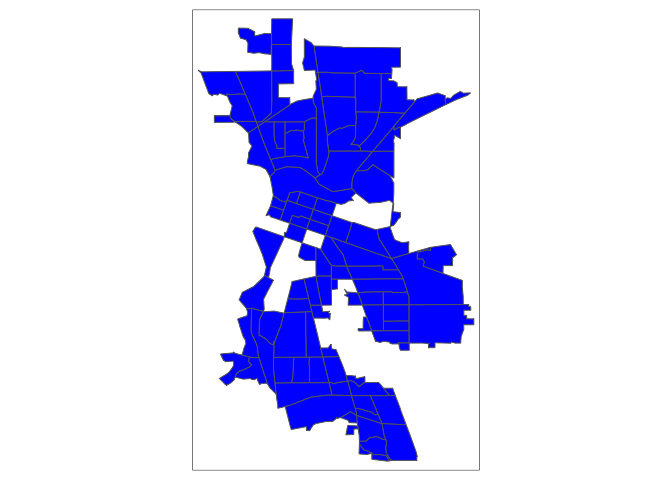

We’ve got permanent holes in Sacramento because we physically removed census tracts with missing values.

One way to keep observations with missing data is to impute a value for missingness. A simple imputation is the mean value of the variable. To impute the mean, we need to use the tidy friendly impute_mean() function in the tidyimpute package. Install this package and load it into R.

install.packages("tidyimpute")
library(tidyimpute)

Then use the function impute_mean(). To use this function, pipe in the data set and then type in the variables you want to impute.

sac.city.tracts.sf.mn <- sac.city.tracts.sf %>%
    impute_mean(psubhous)

Note that you can impute more than one variable within impute_mean() by separating variables with commas. We should now have no missing values

summary(aggr(sac.city.tracts.sf.mn))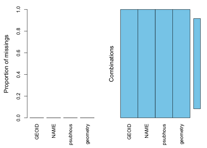

## 
##  Missings per variable: 
##  Variable Count
##     GEOID     0
##      NAME     0
##  psubhous     0
##  geometry     0
## 
##  Missings in combinations of variables: 
##  Combinations Count Percent
##       0:0:0:0   120     100

Therefore allowing us to calculate the mean of psubhous

sac.city.tracts.sf.mn %>% summarize(mean = mean(psubhous))

## Simple feature collection with 1 feature and 1 field
## geometry type:  POLYGON
## dimension:      XY
## bbox:           xmin: -121.5601 ymin: 38.43757 xmax: -121.3627 ymax: 38.6856
## epsg (SRID):    4269
## proj4string:    +proj=longlat +datum=NAD83 +no_defs
##      mean                       geometry
## 1 6.13866 POLYGON ((-121.409 38.50368...

And a Moran’s I

#Turn sac.city.tracts.sf into an sp object.
sac.city.tracts.sp.mn <- as(sac.city.tracts.sf.mn, "Spatial")

sacb.mn<-poly2nb(sac.city.tracts.sp.mn, queen=T)
sacw.mn<-nb2listw(sacb.mn, style="W")
moran.test(sac.city.tracts.sp.mn$psubhous, sacw.mn)

## 
##  Moran I test under randomisation
## 
## data:  sac.city.tracts.sp.mn$psubhous  
## weights: sacw.mn    
## 
## Moran I statistic standard deviate = 1.8814, p-value = 0.02996
## alternative hypothesis: greater
## sample estimates:
## Moran I statistic       Expectation          Variance 
##       0.081778772      -0.008403361       0.002297679

And our map has no holes!!

tmap_mode("view")
tm_shape(sac.city.tracts.sf.mn) +
  tm_polygons(col = "psubhous", style = "quantile")

Other Imputation Methods

The tidyimpute package has a set of functions for imputing missing values in your data. The functions are categorized as univariate and multivariate, where the former imputes a single value for all missing observations (like the mean) whereas the latter imputes a value based on a set of non-missing characteristics. Univariate methods include

impute_max - maximum
impute_minimum - minimum
impute_median - median value
impute_quantile - quantile value
impute_sample - randomly sampled value via bootstrap

Multivariate methods include

impute_fit,impute_predict - use a regression model to predict the value
impute_by_group - use by-group imputation

Some of the multivariate functions may not be fully developed at the moment, but their test versions may be available for download. If you’re looking to use a multivariate method to impute missingness, check the Hmisc and MICE packages.

The MICE package provides functions for imputing missing values using multiple imputation methods. These methods take into account the uncertainty related to the unknown real values by imputing M plausible values for each unobserved response in the data. This renders M different versions of the data set, where the non-missing data is identical, but the missing data entries differ. These methods go beyond the scope of this class, but you can check a number of user created vignettes, include this, this and this. I’ve also uploaded onto Canvas (Additional Readings folder) a chapter from Gelman and Hill that covers missing data.

Website created and maintained by Noli Brazil