Lab 1: Introduction to R
CRD 230 - Spatial Methods in Community Research
Professor Noli Brazil
January 11, 2023
You will be using R to complete all data analysis tasks in this class. For those who have never used R or it has been a long time since you’ve used the program, welcome to what will be a life fulfilling journey!
The objectives of the guide are as follows
- Install and set up R and RStudio.
- Understand R data types
- Understand R data structures
- Understand R functions
- Introduction to tidyverse and its suite of data wrangling functions
- Understand R Markdown
This lab guide follows closely and supplements the material presented in Chapters 2, 4, 5, 7 and 21 in the textbook R for Data Science (RDS).
What is R?
R is a free, open source statistical programming language. It is useful for data cleaning, analysis, and visualization. R is an interpreted language, not a compiled one. This means that you type something into R and it does what you tell it. It is both a command line software and a programming environment. It is an extensible, open-source language and computing environment for Windows, Macintosh, UNIX, and Linux platforms, which allows for the user to freely distribute, study, change, and improve the software. It is basically a free, super big, and complex calculator. You will be using R to accomplish all data analysis tasks in this class. You might be wondering “Why in the world do we need to know how to use a statistical software program?” Here are the main reasons:
You will be learning about abstract concepts in lecture and the readings. Applying these concepts using real data is an important form of learning. A statistical software program is the most efficient (and in many cases the only) means of running data analyses, not just in the cloistered setting of a university classroom, but especially in the real world. Applied data analysis will be the way we bridge statistical theory to the “real world.” And R is the vehicle for accomplishing this.
In order to do applied data analysis outside of the classroom, you need to know how to use a statistical program. There is no way around it as we don’t live in an exclusively pen and paper world. If you want to collect data on soil health, you need a program to store and analyze that data. If you want to collect data on the characteristics of recent migrants, you need a program to store and analyze that data.
The next question you may have is “I love Excel [or insert your favorite program]. Why can’t I use that and forget your stupid R?” Here are some reasons
- it is free. Most programs are not;
- it is open source. Which means the software is community supported. This allows you to get help not from some big corporation (e.g. Microsoft with Excel), but people all around the world who are using R. And R has a lot of users, which means that if you have a problem, and you pose it to the user community, someone will help you;
- it is powerful and extensible (meaning that procedures for analyzing data that don’t currently exist can be readily developed);
- it has the capability for mapping data, an asset not generally available in other statistical software;
- If it isn’t already there, R is becoming the de-facto data analysis tool in the social sciences
R is different from Excel in that it is generally not a point-and-click program. You will be primarily writing code to clean and analyze data. What does writing or sourcing code mean? A basic example will help clarify. Let’s say you are given a dataset with 10 rows representing people living in Davis, CA. You have a variable in the dataset representing individual income. Let’s say this variable is named inc. To get the mean income of the 10 people in your dataset, you would write code that would look something like this
mean(inc)The command tells the program to get the mean of the variable inc. If you wanted the sum, you write the command sum(inc).
Now, where do you write this command? You write it in a script. A script is basically a text file. Think of writing code as something similar to writing an essay in a word document. Instead of sentences to produce an essay, in a programming script you are writing code to run a data analysis. We’ll go through scripting in more detail later in this lab, but the basic process of sourcing code to run a data analysis task is as follows.
- Write code. First, you open your script file, and write code or various commands (like
mean(inc)) that will execute data analysis tasks in this file. - Send code to the software program. You then send some or all of your commands to the statistical software program (R in our case).
- Program produces results based on code. The program then reads in your commands from the file and executes them, spitting out results in its console screen.
I am skipping over many details, most of which are dependent on the type of statistical software program you are using, but the above steps outline the general work flow. You might now be thinking that you’re perfectly happy pointing and clicking your mouse in Excel (or wherever) to do your data analysis tasks. So, why should you adopt the statistical programming approach to conducting a data analysis?
- Your script documents the decisions you made during the data analysis process. This is beneficial for many reasons.
- It allows you to recreate your steps if you need to rerun your analysis many weeks, months or even years in the future.
- It allows you to share your steps with other people. If someone asks you what were the decisions made in the data analysis process, just hand them the script.
- Related to the above points, a script promotes transparency (here is what i did) and reproducibility (you can do it too). When you write code, you are forced to explicitly state the steps you took to do your research. When you do research by clicking through drop-down menus, your steps are lost, or at least documenting them requires considerable extra effort.
- If you make a mistake in a data analysis step, you can go back, change a few lines of code, and poof, you’ve fixed your problem.
- It is more efficient. In particular, cleaning data can encompass a lot of tedious work that can be streamlined using statistical programming.
Hopefully, I’ve convinced you that statistical programming and R are worthwhile to learn.
Getting R
R can be downloaded from one of the “CRAN” (Comprehensive R Archive Network) sites. In the US, the main site is at http://cran.us.r-project.org/. Look in the “Download and Install R” area. Click on the appropriate link based on your operating system.
If you already have R on your computer, make sure you have the most updated version of R on your personal computer (4.2.2 “Innocent and Trusting”).
Mac OS X
On the “R for Mac OS X” page, there are multiple packages that could be downloaded. If you are running High Sierra or higher, click on R-4.2.2.pkg; if you are running an earlier version of OS X, download the appropriate version listed under “Binary for legacy OS X systems.”
After the package finishes downloading, locate the installer on your hard drive, double-click on the installer package, and after a few screens, select a destination for the installation of the R framework (the program) and the R.app GUI. Note that you will have to supply the Administrator’s password. Close the window when the installation is done.
An application will appear in the Applications folder: R.app.
Browse to the XQuartz download page. Click on the most recent version of XQuartz to download the application.
Run the XQuartz installer. XQuartz is needed to create windows to display many types of R graphics: this used to be included in MacOS until version 10.8 but now must be downloaded separately.
Windows
On the “R for Windows” page, click on the “base” link, which should take you to the “R-4.2.2 for Windows (32/64 bit)” page
On this page, click “Download R 4.2.2 for Windows”, and save the exe file to your hard disk when prompted. Saving to the desktop is fine.
To begin the installation, double-click on the downloaded file. Don’t be alarmed if you get unknown publisher type warnings. Window’s User Account Control will also worry about an unidentified program wanting access to your computer. Click on “Run”.
Select the proposed options in each part of the install dialog. When the “Select Components” screen appears, just accept the standard choices
Note: Depending on the age of your computer and version of Windows, you may be running either a “32-bit” or “64-bit” version of the Windows operating system. If you have the 64-bit version (most likely), R will install the appropriate version (R x64 3.5.2) and will also (for backwards compatibility) install the 32-bit version (R i386 3.5.2). You can run either, but you will probably just want to run the 64-bit version.
What is RStudio?
If you click on the R program you just downloaded, you will find a very basic user interface. For example, below is what I get on a Mac

We will not use R’s direct interface to run analyses. Instead, we will use the program RStudio. RStudio gives you a true integrated development environment (IDE), where you can write code in a window, see results in other windows, see locations of files, see objects you’ve created, and so on. To clarify which is which: R is the name of the programming language itself and RStudio is a convenient interface.
Getting RStudio
To download and install RStudio, follow the directions below
- Navigate to RStudio’s download site
- Click on the appropriate link based on your OS (Windows, Mac, Linux and many others). Do not download anything from the “Zip/Tarballs” section.
- Click on the installer that you downloaded. Follow the installation wizard’s directions, making sure to keep all defaults intact. After installation, RStudio should pop up in your Applications or Programs folder/menu.
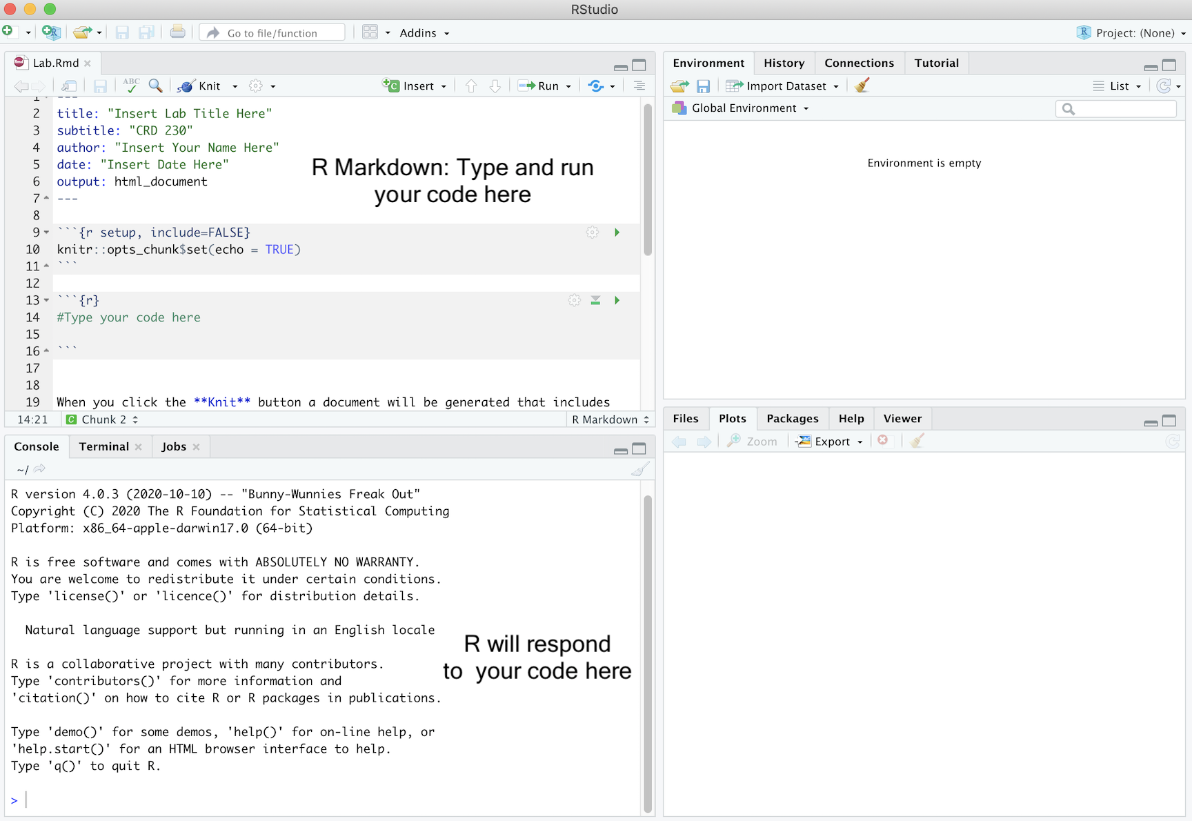
The RStudio Interface
Open up RStudio. You should see the interface shown in the figure below which has three windows.
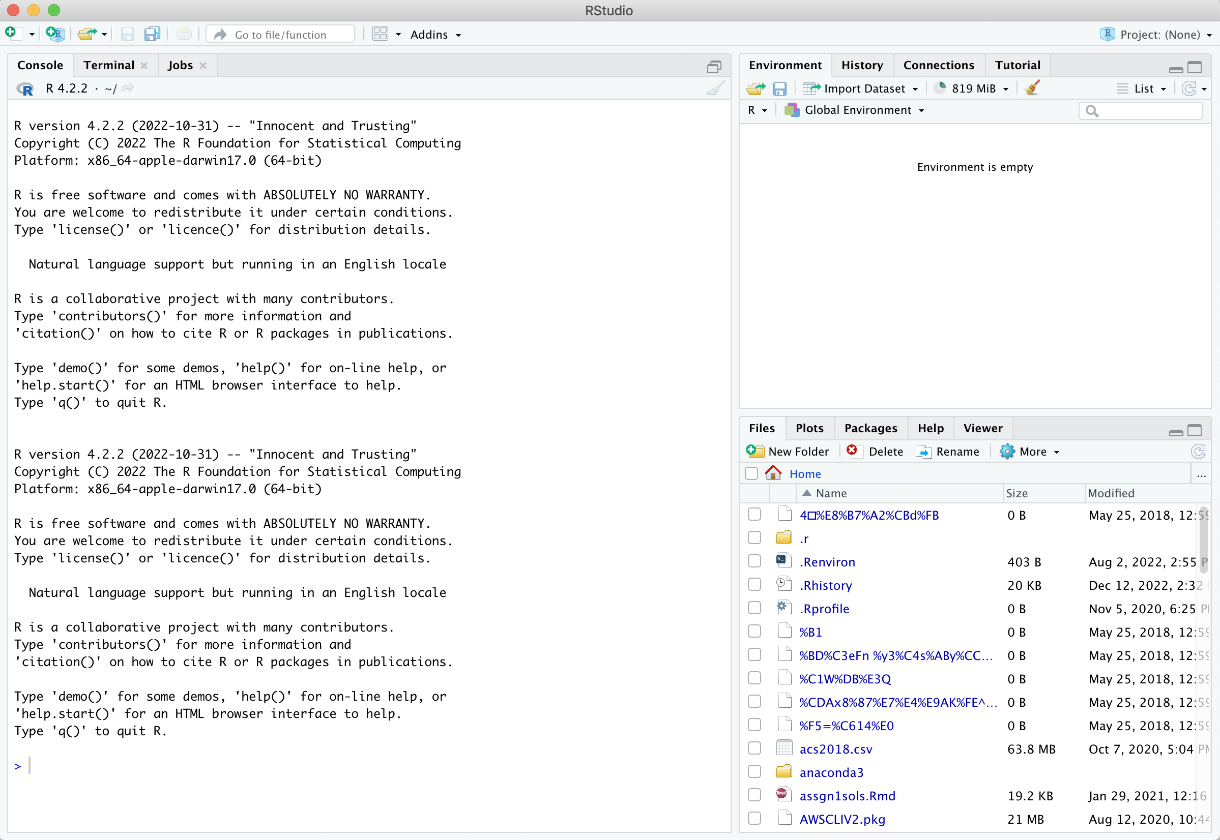
The RStudio Interface.
- Console (left) - The way R works is you write a line of code to execute some kind of task on a data object. The R Console allows you to run code interactively. The screen prompt
>is an invitation from R to enter its world. This is where you type code in, press enter to execute the code, and see the results. - Environment, History, and Connections tabs (upper-right)
- Environment - shows all the R objects that are currently open in your workspace. This is the place, for example, where you will see any data you’ve loaded into R. When you exit RStudio, R will clear all objects in this window. You can also click on
 to clear out all the objects loaded and created in your current session.
 - History - shows a list of executed commands in the current session.
- Connections - you can connect to a variety of data sources, and explore the objects and data inside the connection. I typically don’t use this window, but you can.
- Environment - shows all the R objects that are currently open in your workspace. This is the place, for example, where you will see any data you’ve loaded into R. When you exit RStudio, R will clear all objects in this window. You can also click on
- Files, Plots, Packages, Help and Viewer tabs (lower-right)
- Files - shows all the files and folders in your current working directory (more on what this means later).
- Plots - shows any charts, graphs, maps and plots you’ve successfully executed.
- Packages - tells you all the R packages that you have access to (more on this later).
- Help - shows help documentation for R commands that you’ve called up.
- Viewer - allows you to view local web content (won’t be using this much).
There is actually fourth window. But, we’ll get to this window a little later (if you read the assignment guidelines you already know what this fourth window is).
Setting RStudio Defaults
While not required, I strongly suggest that you change preferences in RStudio to never save the workspace so you always open with a clean environment. See Ch. 8.1 of R4DS for some more background
- From the Tools menu on RStudio, open the Tools menu and then select Global Options.
- If not already highlighted, click on the General button from the left panel.
- Uncheck the following Restore boxes
- Restore most recently opened project at startup
- Restore previously open source documents at startup
- Restore .RData into workspace at startup
- Set Save Workspace to .RData on exit to Never
- Click OK at the bottom to save the changes and close the preferences window. You may need to restart RStudio.

The reason for making these changes is that it is preferable for reproducibility to start each R session with a clean environment. You can restore a previous environment either by rerunning code or by manually loading a previously saved session.
The R Studio environment is modified when you execute code from files or from the console. If you always start fresh, you do not need to be concerned about things not working because of something you typed in the console, but did not save in a file.
You only need to set these preferences once.
R Data Types
Let’s now explore what R can do. R is really just a big fancy calculator. For example, type in the following mathematical expression in the R console (left window)
1+1## [1] 2Note that spacing does not matter: 1+1 will generate the same answer as 1 + 1. Can you say hello to the world?
hello world## Error: <text>:1:7: unexpected symbol
## 1: hello world
## ^Nope. What is the problem here? We need to put quotes around it.
"hello world"## [1] "hello world"“hello world” is a character and R recognizes characters only if there are quotes around it. This brings us to the topic of basic data types in R. There are four basic data types in R: character, logical, numeric, and factors (there are two others - complex and raw - but we won’t cover them because they are rarely used in practice).
Characters
Characters are used to represent words or letters in R. We saw this above with “hello world”. Character values are also known as strings. You might think that the value "1" is a number. Well, with quotes around, it isn’t! Anything with quotes will be interpreted as a character. No ifs, ands or buts about it.
Logicals
A logical takes on two values: FALSE or TRUE. Logicals are usually constructed with comparison operators, which we’ll go through more carefully in Lab 2. Think of a logical as the answer to a question like “Is this value greater than (lower than/equal to) this other value?” The answer will be either TRUE or FALSE. TRUE and FALSE are logical values in R. For example, typing in the following
3 > 2## [1] TRUEGives you a true. What about the following?
"jacob" == "catherine"## [1] FALSENumeric
Numerics are separated into two types: integer and double. The distinction between integers and doubles is usually not important. R treats numerics as doubles by default because it is a less restrictive data type. You can do any mathematical operation on numeric values. We added one and one above. We can also multiply using the * operator.
2*3## [1] 6Divide
4/2## [1] 2And even take the logarithm!
log(1)## [1] 0log(0)## [1] -InfUh oh. What is -Inf? Well, you can’t take the logarithm of 0, so R is telling you that you’re getting a non numeric value in return. The value -Inf is another type of value type that you can get in R.
Factors
Think of a factor as a categorical variable. It is sort of like a character, but not really. It is actually a numeric code with character-valued levels. Think of a character as a true string and a factor as a set of categories represented as characters. We won’t use factors too much in this course.
R Data Structures
You just learned that R has four basic data types. Now, let’s go through how we can store data in R. That is, you type in the character “hello world” or the number 3, and you want to store these values. You do this by using R’s various data structures.
Vectors
A vector is the most common and basic R data structure and is pretty much the workhorse of the language. A vector is simply a sequence of values which can be of any data type but all of the same type. There are a number of ways to create a vector depending on the data type, but the most common is to insert the data you want to save in a vector into the command c(). For example, to represent the values 4, 16 and 9 in a vector type in
c(4, 16, 9)## [1] 4 16 9You can also have a vector of character values
c("jacob", "anne", "gwen")## [1] "jacob" "anne" "gwen"The above code does not actually “save” the values 4, 16, and 9 - it just presents it on the screen in a vector. If you want to use these values again without having to type out c(4, 16, 9), you can save it in a data object. At the heart of almost everything you will do (or ever likely to do) in R is the concept that everything in R is an object. These objects can be almost anything, from a single number or character string (like a word) to highly complex structures like the output of a plot, a map, a summary of your statistical analysis or a set of R commands that perform a specific task.
You assign data to an object using the arrow sign <-. This will create an object in R’s memory that can be called back into the command window at any time. For example, you can save “hello world” to a vector called b by typing in
b <- "hello world"
b
## [1] "hello world"You can pronounce the above as “b becomes ‘hello world’”.
Note that R is case sensitive, if you type in B instead of b, you will get an error.
Similarly, you can save the numbers 4, 16 and 9 into a vector called v1
v1 <- c(4, 16, 9)
v1
## [1] 4 16 9You should see the objects b and v1 pop up in the Environment tab on the top right window of your RStudio interface.
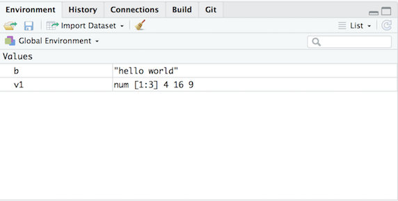
Environment window
Note that the name v1 is nothing special here. You could have named the object x or crd230 or your pet’s name (mine was charlie). You can’t, however, name objects using special characters (e.g. !, @, $) or only numbers (although you can combine numbers and letters, but a number cannot be at the beginning e.g. 2d2). For example, you’ll get an error if you save the vector c(4,16,9) to an object with the following names
123 <- c(4, 16, 9)
!!! <- c(4, 16, 9)
## Error: <text>:2:5: unexpected assignment
## 1: 123 <- c(4, 16, 9)
## 2: !!! <-
## ^Also note that to distinguish a character value from a variable name, it needs to be quoted. “v1” is a character value whereas v1 is a variable. One of the most common mistakes for beginners is to forget the quotes.
brazil## Error in eval(expr, envir, enclos): object 'brazil' not foundThe error occurs because R tries to print the value of object brazil, but there is no such variable. So remember that any time you get the error message object 'something' not found, the most likely reason is that you forgot to quote a character value. If not, it probably means that you have misspelled, or not yet created, the object that you are referring to. I’ve included the common pitfalls and R tips in this class resource.
Every vector has two key properties: type and length. The type property indicates the data type that the vector is holding. Use the command typeof() to determine the type
typeof(b)## [1] "character"typeof(v1)## [1] "double"Note that a vector cannot hold values of different types. If different data types exist, R will coerce the values into the highest type based on its internal hierarchy: logical < integer < double < character. Type in test <- c("r", 6, TRUE) in your R console. What is the vector type of test?
The command length() determines the number of data values that the vector is storing
length(b)## [1] 1length(v1)## [1] 3You can also directly determine if a vector is of a specific data type by using the command is.X() where you replace X with the data type. For example, to find out if v1 is numeric, type in
is.numeric(b)## [1] FALSEis.numeric(v1)## [1] TRUEThere is also is.logical(), is.character(), and is.factor(). You can also coerce a vector of one data type to another. For example, save the value “1” and “2” (both in quotes) into a vector named x1
x1 <- c("1", "2")
typeof(x1)
## [1] "character"To convert x1 into a numeric, use the command as.numeric()
x2 <- as.numeric(x1)
typeof(x2)
## [1] "double"There is also as.logical(), as.character(), and as.factor().
An important practice you should adopt early is to keep only necessary objects in your current R Environment. For example, we will not be using x2 any longer in this guide. To remove this object from R forever, use the command rm()
rm(x2)The data frame object x2 should have disappeared from the Environment tab. Bye bye!
Also note that when you close down R Studio, the objects you created above will disappear for good. Unless you save them onto your hard drive (we’ll touch on saving data in Lab 2), all data objects you create in your current R session will go bye bye when you exit the program.
Data Frames
We learned that data values can be stored in data structures known as vectors. The next step is to learn how to store vectors into an even higher level data structure. The data frame can do this. Data frames store vectors of the same length. Create a vector called v2 storing the values 5, 12, and 25
v2 <- c(5,12,25)We can create a data frame using the command data.frame() storing the vectors v1 and v2 as columns
data.frame(v1, v2)## v1 v2
## 1 4 5
## 2 16 12
## 3 9 25Store this data frame in an object called df1
df1<-data.frame(v1, v2)df1 should pop up in your Environment window. You’ll notice a  next to df1. This tells you that df1 possesses or holds more than one object. Click on and you’ll see the two vectors we saved into df1. Another neat thing you can do is directly click on df1 from the Environment window to bring up an Excel style worksheet on the top left of your RStudio interface. You can also type in
View(df1)to bring the worksheet up. You can’t edit this worksheet directly, but it allows you to see the values that a higher level R data object contains.
We can store different types of vectors in a data frame. For example, we can store one character vector and one numeric vector in a single data frame.
v3 <- c("jacob", "anne", "gwen")
df2 <- data.frame(v1, v3)
df2
## v1 v3
## 1 4 jacob
## 2 16 anne
## 3 9 gwenFor higher level data structures like a data frame, use the function class() to figure out what kind of object you’re working with.
class(df2)## [1] "data.frame"We can’t use length() on a data frame because it has more than one vector. Instead, it has dimensions - the number of rows and columns. You can find the number of rows and columns that a data frame has by using the command dim()
dim(df1)## [1] 3 2Here, the data frame df1 has 3 rows and 2 columns. Data frames also have column names, which are characters.
colnames(df1)## [1] "v1" "v2"In this case, the data frame used the vector names for the column names.
We can extract columns from data frames by referring to their names using the $ sign.
df1$v1## [1] 4 16 9We can also extra data from data frames using brackets [ , ]
df1[,1]## [1] 4 16 9The value before the comma indicates the row, which you leave empty if you are not selecting by row, which we did above. The value after the comma indicates the column, which you leave empty if you are not selecting by column. The above line of code selected the first column. Let’s select the 2nd row.
df1[2,]## v1 v2
## 2 16 12What is the value in the 2nd row and 1st column?
df1[2,1]## [1] 16Functions
Let’s take a step back and talk about functions (also known as commands). An R function is a packaged recipe that converts one or more inputs (called arguments) into a single output. You execute all of your tasks in R using functions. We have already used a couple of functions above including typeof() and colnames(). Every function in R will have the following basic format
functionName(arg1 = val1, arg2 = val2, ...)
In R, you type in the function’s name and set a number of options or parameters within parentheses that are separated by commas. Some options need to be set by the user - i.e. the function will spit out an error because a required option is blank - whereas others can be set but are not required because there is a default value established.
Let’s use the function seq() which makes regular sequences of numbers. You can find out what the options are for a function by calling up its help documentation by typing ? and the function name
? seqThe help documentation should have popped up in the bottom right window of your RStudio interface. The documentation should also provide some examples of the function at the bottom of the page. Type the arguments from = 1, to = 10 inside the parentheses
seq(from = 1, to = 10)## [1] 1 2 3 4 5 6 7 8 9 10You should get the same result if you type in
seq(1, 10)## [1] 1 2 3 4 5 6 7 8 9 10The code above demonstrates something about how R resolves function arguments. When you use a function, you can always specify all the arguments in arg = value form. But if you do not, R attempts to resolve by position. So in the code above, it is assumed that we want a sequence from = 1 that goes to = 10 because we typed 1 before 10. Type in 10 before 1 and see what happens. Since we didn’t specify step size, the default value of by in the function definition is used, which ends up being 1 in this case.
Each argument requires a certain type of data type. For example, you’ll get an error when you use character values in seq()
seq("p", "w")## Error in seq.default("p", "w"): 'from' must be a finite numberPackages
Functions do not exist in a vacuum, but exist within R packages. Packages are the fundamental units of reproducible R code. They include reusable R functions, the documentation that describes how to use them, and sample data. At the top left of a function’s help documentation, you’ll find in curly brackets the R package that the function is housed in. For example, type in your console ? seq. At the top right of the help documentation, you’ll find that seq() is in the package base. All the functions we have used so far are part of packages that have been pre-installed and pre-loaded into R.
In order to use functions in a new package, you first need to install the package using the install.packages() command. For example, we will be using commands from the package tidyverse in this lab. If you are working on a campus lab computer, you will likely not need to install this package.
install.packages("tidyverse")You should see a bunch of gobbledygook roll through your console screen. Don’t worry, that’s just R downloading all of the other packages and applications that tidyverse relies on. These are known as dependencies. Unless you get a message in red that indicates there is an error (like we saw when we typed in “hello world” without quotes), you should be fine.
Next, you will need to load packages in your working environment (every time you start RStudio). We do this with the library() function. Notice there are no quotes around tidyverse this time.
library(tidyverse)The Packages window at the lower-right of your RStudio shows you all the packages you currently have installed. If you don’t have a package listed in this window, you’ll need to use the install.packages() function to install it. If the package is checked, that means it is loaded into your current R session
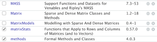
For example, here is a section of my Packages window
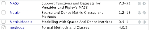
The only packages loaded into my current session is methods, a package that is loaded every time you open an R session. Let’s say I use install.packages() to install the package matrixStats. The window now looks like
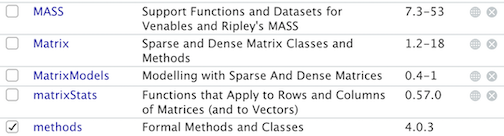
When you load it in using library(), a check mark appears next to matrixStats
To uninstall a package, use the function remove.packages().
Note that you only need to install packages once (install.pacakges()), but you need to load them each time you relaunch RStudio (library()). Repeat after me: Install once, library every time. If you need to reinstall R or update to a new version of R, you will need to reinstall all packages. And as noted earlier, R has several packages already preloaded into your working environment. These are known as base packages and a list of their functions can be found here.
Tidyverse
In most labs, we will be using commands from the tidyverse package. Tidyverse is a collection of high-powered, consistent, and easy-to-use packages developed by a number of thoughtful and talented R developers.The consistency of the tidyverse, together with the goal of increasing productivity, mean that the syntax of tidy functions is typically straightforward to learn. You can read more about tidyverse principles in Chapter 9, pages 147-151 in RDS.
Excited about entering the tidyverse? I bet you are, so here is a badge to show your excitement!
Tibbles
Although the tidyverse works with all data objects, its fundamental object type is the tibble. Tibbles are data frames, but they tweak some older behaviors to make life a little easier. There are two main differences in the usage of a data frame vs a tibble: printing and subsetting. Let’s be clear here - tibbles are just a special kind of data frame. They just makes things a little “tidier.” Let’s bring in some data to illustrate the differences and similarities between data frames and tibbles. Install the package nycflights13
install.packages("nycflights13") Make sure you also load the package.
library(nycflights13)There is a dataset called flights included in this package. It includes information on all 336,776 flights that departed from New York City in 2013. Let’s save this file in the local R environment
nyctib <- flights
class(nyctib)
## [1] "tbl_df" "tbl" "data.frame"This dataset is a tibble. Let’s also save it as a regular data frame by using the as.data.frame() function
nycdf <- as.data.frame(flights)
class(nycdf)
## [1] "data.frame"The first difference between data frames and tibbles is how the dataset looks. Tibbles have a refined print method that shows only the first 10 rows, and only the columns that fit on the screen. In addition, each column reports its name and type.
nyctib## # A tibble: 336,776 × 19
## year month day dep_time sched_de…¹ dep_d…² arr_t…³ sched…⁴ arr_d…⁵ carrier
## <int> <int> <int> <int> <int> <dbl> <int> <int> <dbl> <chr>
## 1 2013 1 1 517 515 2 830 819 11 UA
## 2 2013 1 1 533 529 4 850 830 20 UA
## 3 2013 1 1 542 540 2 923 850 33 AA
## 4 2013 1 1 544 545 -1 1004 1022 -18 B6
## 5 2013 1 1 554 600 -6 812 837 -25 DL
## 6 2013 1 1 554 558 -4 740 728 12 UA
## 7 2013 1 1 555 600 -5 913 854 19 B6
## 8 2013 1 1 557 600 -3 709 723 -14 EV
## 9 2013 1 1 557 600 -3 838 846 -8 B6
## 10 2013 1 1 558 600 -2 753 745 8 AA
## # … with 336,766 more rows, 9 more variables: flight <int>, tailnum <chr>,
## # origin <chr>, dest <chr>, air_time <dbl>, distance <dbl>, hour <dbl>,
## # minute <dbl>, time_hour <dttm>, and abbreviated variable names
## # ¹sched_dep_time, ²dep_delay, ³arr_time, ⁴sched_arr_time, ⁵arr_delayTibbles are designed so that you don’t overwhelm your console when you print large data frames. Compare the print output above to what you get with a data frame
nycdfUgly, right? You can bring up the Excel like worksheet of the tibble (or data frame) using the View() function
View(nyctib)You can identify the names of the columns (and hence the variables in the dataset) by using the function names()
names(nyctib)## [1] "year" "month" "day" "dep_time"
## [5] "sched_dep_time" "dep_delay" "arr_time" "sched_arr_time"
## [9] "arr_delay" "carrier" "flight" "tailnum"
## [13] "origin" "dest" "air_time" "distance"
## [17] "hour" "minute" "time_hour"Finally, you can convert a regular data frame to a tibble using the as_tibble() function
as_tibble(nycdf)## # A tibble: 336,776 × 19
## year month day dep_time sched_de…¹ dep_d…² arr_t…³ sched…⁴ arr_d…⁵ carrier
## <int> <int> <int> <int> <int> <dbl> <int> <int> <dbl> <chr>
## 1 2013 1 1 517 515 2 830 819 11 UA
## 2 2013 1 1 533 529 4 850 830 20 UA
## 3 2013 1 1 542 540 2 923 850 33 AA
## 4 2013 1 1 544 545 -1 1004 1022 -18 B6
## 5 2013 1 1 554 600 -6 812 837 -25 DL
## 6 2013 1 1 554 558 -4 740 728 12 UA
## 7 2013 1 1 555 600 -5 913 854 19 B6
## 8 2013 1 1 557 600 -3 709 723 -14 EV
## 9 2013 1 1 557 600 -3 838 846 -8 B6
## 10 2013 1 1 558 600 -2 753 745 8 AA
## # … with 336,766 more rows, 9 more variables: flight <int>, tailnum <chr>,
## # origin <chr>, dest <chr>, air_time <dbl>, distance <dbl>, hour <dbl>,
## # minute <dbl>, time_hour <dttm>, and abbreviated variable names
## # ¹sched_dep_time, ²dep_delay, ³arr_time, ⁴sched_arr_time, ⁵arr_delayNot all functions work with tibbles, particularly those that are specific to spatial data. As such, we’ll be using a combination of tibbles and regular data frames throughout the class, with a preference towards tibbles where possible. Note that when you search on Google for how to do something in R, you will likely get non tidy ways of doing things. Most of these suggestions are fine, but some are not and may screw you up down the road. My advice is to try to stick with tidy functions to do things in R.
Anyway, you earned another badge. Yes!

Data Wrangling
It is rare that the data work on are in exactly the right form for analysis. For example, you might want to discard certain variables from the dataset to reduce clutter. Or you need to create new variables from existing ones. Or you encounter missing data. The process of gathering data in its raw form and molding it into a form that is suitable for its end use is known as data wrangling. What’s great about the tidyverse package is its suite of functions make data wrangling relatively easy, straight forward, and transparent.
In this lab, we won’t have time to go through all of the methods and functions in R that are associated with the data wrangling process. We will cover more in later labs and many methods you will have to learn on your own given the specific tasks you will need to accomplish. In the rest of this guide, we’ll go through some of the basic data wrangling techniques using the functions found in the package dplyr, which was automatically installed and loaded when you brought in the tidyverse package. These functions can be used for either tibbles or regular data frames.
Reading in data
The dataset nycflights13 was included in an R package. In most cases, you’ll have to read it in. Most data files you will encounter are comma-delimited (or comma-separated) files, which have .csv extensions. Comma-delimited means that columns are separated by commas. We’re going to bring in two csv files lab1dataset1.csv and lab1dataset2.csv. The first file is a county-level dataset containing median household income. The second file is also a county-level dataset containing Non-Hispanic white, Non-Hispanic black, non-Hispanic Asian, and Hispanic population counts. Both data sets come from the 2014-2018 American Community Survey (ACS). We’ll cover the Census, and how to download Census data, in the next lab.
To read in a csv file, use the function read_csv(), which is a part of the tidyverse package, and plug in the name of the file in quotes inside the parentheses. Make sure you include the .csv extension. I uploaded the two files on GitHub, so you can read them in directly from there. We’ll name these objects ca1 and ca2
ca1 <- read_csv("https://raw.githubusercontent.com/crd230/data/master/lab1dataset1.csv")
ca2 <- read_csv("https://raw.githubusercontent.com/crd230/data/master/lab1dataset2.csv")
You should see two tibbles ca1 and ca2 pop up in your Environment window (top right). Every time you bring a dataset into R for the first time, look at it to make sure you understand its structure. You can do this a number of ways. One is to use the function glimpse(), which gives you a succinct summary of your data.
glimpse(ca1)## Rows: 58
## Columns: 4
## $ `FIPS Code` <dbl> 6071, 602…
## $ County <chr> "San Bern…
## $ `Formatted FIPS` <chr> "06071", …
## $ `Estimated median income of a household, between 2014-2018.` <dbl> 60164, 52…glimpse(ca2)## Rows: 58
## Columns: 12
## $ GEOID <chr> "06033", "06047", "06043", "06049", "06013", "06027", "06099"…
## $ NAME <chr> "Lake County, California", "Merced County, California", "Mari…
## $ tpoprE <dbl> 64148, 269075, 17540, 8938, 1133247, 18085, 539301, 443738, 1…
## $ tpoprM <dbl> NA, NA, NA, NA, NA, NA, NA, NA, NA, NA, NA, NA, NA, NA, NA, N…
## $ nhwhiteE <dbl> 45623, 76008, 14125, 6962, 502951, 11389, 229796, 199356, 923…
## $ nhwhiteM <dbl> 30, 200, 31, 6, 607, 26, 445, 221, 121, 38, 980, 166, 201, 48…
## $ nhblkE <dbl> 1426, 8038, 166, 149, 93683, 160, 14338, 7881, 40, 434, 14400…
## $ nhblkM <dbl> 112, 371, 111, 97, 1433, 37, 584, 449, 47, 88, 2016, 209, 438…
## $ nhasnE <dbl> 642, 19487, 243, 130, 182135, 289, 28599, 22996, 336, 1705, 2…
## $ nhasnM <dbl> 187, 630, 95, 118, 1993, 62, 876, 507, 223, 125, 1893, 402, 6…
## $ hispE <dbl> 12830, 158494, 1909, 1292, 288101, 3927, 245973, 200060, 3866…
## $ hispM <dbl> NA, NA, NA, NA, NA, NA, NA, NA, NA, NA, NA, NA, NA, NA, NA, N…If you like viewing your data through an Excel style worksheet, type in View(ca1), and ca1 should pop up in the top left window of your R Studio interface. Scroll up and down, left and right.
We’ll learn how to summarize your data using descriptive statistics and graphs in the next lab.
By learning how to read in data the tidy way, you’ve earned another badge! Hooray!

Renaming variables
You will likely encounter a variable with a name that is not descriptive. The more descriptive the variable names, the more efficient your analysis will be and the less likely you are going to make a mistake. To see the names of variables in your dataset, use the names() command.
names(ca1)## [1] "FIPS Code"
## [2] "County"
## [3] "Formatted FIPS"
## [4] "Estimated median income of a household, between 2014-2018."The name Estimated median income of a household, between 2014-2018. is super duper long! Use the command rename() to - what else? - rename a variable! Let’s rename Estimated median income of a household, between 2014-2018. to medinc.
rename(ca1, medinc = "Estimated median income of a household, between 2014-2018.")## # A tibble: 58 × 4
## `FIPS Code` County `Formatted FIPS` medinc
## <dbl> <chr> <chr> <dbl>
## 1 6071 San Bernardino 06071 60164
## 2 6027 Inyo 06027 52874
## 3 6029 Kern 06029 52479
## 4 6093 Siskiyou 06093 44200
## 5 6065 Riverside 06065 63948
## 6 6019 Fresno 06019 51261
## 7 6035 Lassen 06035 56362
## 8 6049 Modoc 06049 45149
## 9 6107 Tulare 06107 47518
## 10 6023 Humboldt 06023 45528
## # … with 48 more rowsNote that you can rename multiple variables within the same rename() command. For example, we can also rename Formatted FIPS to GEOID. Make this permanent by assigning it back to ca1 using the arrow operator <-
ca1 <- rename(ca1, medinc = "Estimated median income of a household, between 2014-2018.",
                 GEOID = "Formatted FIPS")
names(ca1)
## [1] "FIPS Code" "County" "GEOID" "medinc"Selecting variables
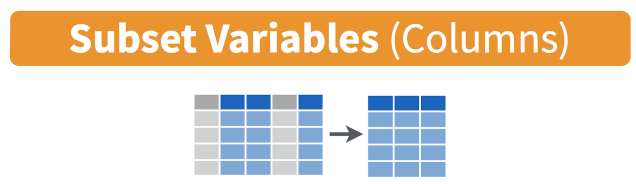
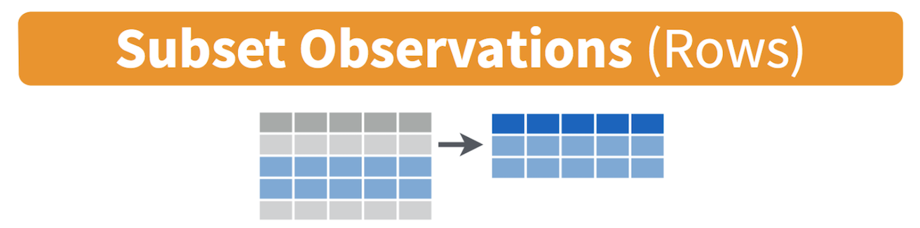
In practice, most of the data files you will download will contain variables you don’t need. It is easier to work with a smaller dataset as it reduces clutter and clears up memory space, which is important if you are executing complex tasks on a large number of observations. Use the command select() to keep variables by name. Visually, we are doing the following (taken from the RStudio cheatsheet)
Let’s take a look at the variables we have in the ca2 dataset
names(ca2)## [1] "GEOID" "NAME" "tpoprE" "tpoprM" "nhwhiteE" "nhwhiteM"
## [7] "nhblkE" "nhblkM" "nhasnE" "nhasnM" "hispE" "hispM"We’ll go into more detail what these variables mean next lab when we cover the U.S. Census, but we only want to keep the variables GEOID, which is the county FIPS code (a unique numeric identifier), and tpoprE, nhwhiteE, nhblkE, nhasnE, and hispE, which are the total, white, black, Asian and Hispanic population counts.
ca2 <- select(ca2, GEOID, tpoprE, nhwhiteE, nhblkE, nhasnE, hispE)Here, we provide the data object first, followed by the variables we want to keep separated by commas.
Let’s keep County, GEOID, and medinc from the ca1 dataset. Rather than listing all the variables we want to keep like we did above, a shortcut way of doing this is to use the : operator.
select(ca1, County:medinc)## # A tibble: 58 × 3
## County GEOID medinc
## <chr> <chr> <dbl>
## 1 San Bernardino 06071 60164
## 2 Inyo 06027 52874
## 3 Kern 06029 52479
## 4 Siskiyou 06093 44200
## 5 Riverside 06065 63948
## 6 Fresno 06019 51261
## 7 Lassen 06035 56362
## 8 Modoc 06049 45149
## 9 Tulare 06107 47518
## 10 Humboldt 06023 45528
## # … with 48 more rowsThe : operator tells R to select all the variables from County to medinc. This operator is useful when you’ve got a lot of variables to keep and they all happen to be ordered sequentially.
You can use also use select() command to keep variables except for the ones you designate. For example, to keep all variables in ca1 except FIPS Code and save this back into ca1, type in
ca1 <- select(ca1, -"FIPS Code")The negative sign tells R to exclude the variable. Notice we need to use quotes around FIPS Code because it contains a space. You can delete multiple variables. For example, if you wanted to keep all variables except FIPS Code and County, you would type in select(ca1, -"FIPS Code", -County).
Take a glimpse to see if we got what we wanted.
glimpse(ca1)## Rows: 58
## Columns: 3
## $ County <chr> "San Bernardino", "Inyo", "Kern", "Siskiyou", "Riverside", "Fre…
## $ GEOID <chr> "06071", "06027", "06029", "06093", "06065", "06019", "06035", …
## $ medinc <dbl> 60164, 52874, 52479, 44200, 63948, 51261, 56362, 45149, 47518, …Do the same for ca2.
Creating new variables
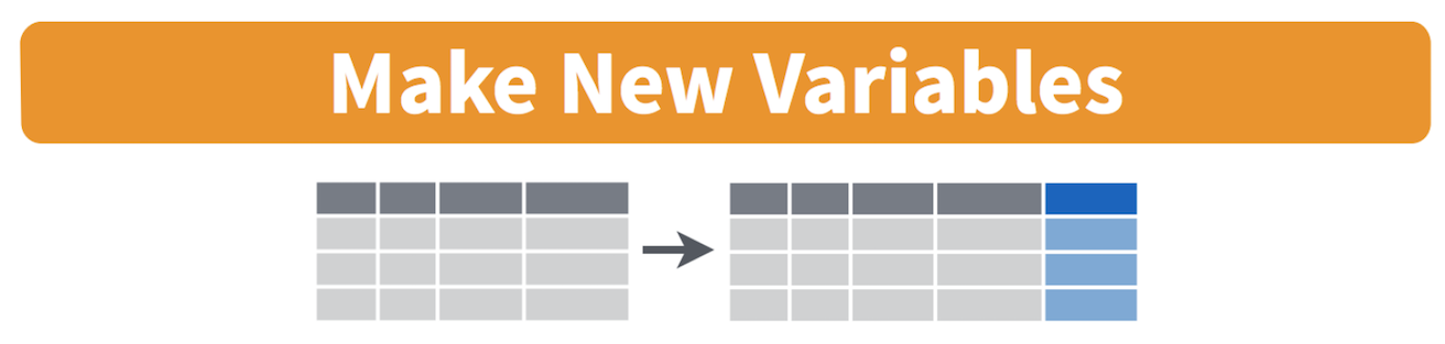
The mutate() function allows you to create new variables within your dataset. This is important when you need to transform variables in some way - for example, calculating a ratio or adding two variables together. Visually, you are doing this
You can use the mutate() command to generate as many new variables as you would like. For example, let’s construct four new variables in ca2 - the percent of residents who are non-Hispanic white, non-Hispanic Asian, non-Hispanic black, and Hispanic. Name these variables pwhite, pasian, pblack, and phisp, respectively.
mutate(ca2, pwhite = nhwhiteE/tpoprE, pasian = nhasnE/tpoprE,
              pblack = nhblkE/tpoprE, phisp = hispE/tpoprE)
Note that you can create new variables based on the variables you just created in the same line of code. For example, you can create a categorical variable yielding “Majority” if the tract is majority Hispanic and “Not Majority” otherwise after creating the percent Hispanic variable within the same mutate() command. Let’s save these changes back into ca2.
ca2 <- mutate(ca2, pwhite = nhwhiteE/tpoprE, pasian = nhasnE/tpoprE,
              pblack = nhblkE/tpoprE, phisp = hispE/tpoprE,
              mhisp = case_when(phisp > 0.5 ~ "Majority",
                                TRUE ~ "Not Majority"))
We used the function case_when() to create mhisp - the function tells R that if the condition phisp > 0.5 is met, the tract’s value for the variable mhisp will be “Majority”, otherwise (designated by TRUE) it will be “Not Majority”.
Take a look at our data
glimpse(ca2)## Rows: 58
## Columns: 11
## $ GEOID <chr> "06033", "06047", "06043", "06049", "06013", "06027", "06099"…
## $ tpoprE <dbl> 64148, 269075, 17540, 8938, 1133247, 18085, 539301, 443738, 1…
## $ nhwhiteE <dbl> 45623, 76008, 14125, 6962, 502951, 11389, 229796, 199356, 923…
## $ nhblkE <dbl> 1426, 8038, 166, 149, 93683, 160, 14338, 7881, 40, 434, 14400…
## $ nhasnE <dbl> 642, 19487, 243, 130, 182135, 289, 28599, 22996, 336, 1705, 2…
## $ hispE <dbl> 12830, 158494, 1909, 1292, 288101, 3927, 245973, 200060, 3866…
## $ pwhite <dbl> 0.7112147, 0.2824789, 0.8053022, 0.7789215, 0.4438141, 0.6297…
## $ pasian <dbl> 0.010008106, 0.072422187, 0.013854048, 0.014544641, 0.1607195…
## $ pblack <dbl> 0.022229843, 0.029872712, 0.009464082, 0.016670396, 0.0826677…
## $ phisp <dbl> 0.20000624, 0.58903280, 0.10883694, 0.14455135, 0.25422613, 0…
## $ mhisp <chr> "Not Majority", "Majority", "Not Majority", "Not Majority", "…Joining tables
Rather than working on two separate datasets, we should join the two datasets ca1 and ca2, because we may want to examine the relationship between median household income, which is in ca1, and racial/ethnic composition, which is in ca2. To do this, we need a unique ID that connects the tracts across the two files. The unique Census ID for a county combines the county and state IDs. The Census ID is named GEOID in both files. The IDs should be the same data class, which is the case.
class(ca1$GEOID)## [1] "character"class(ca2$GEOID)## [1] "character"If they are not the same class, we can coerce them using the as.numeric() or as.character() function described earlier.
To merge the datasets together, use the function left_join(), which matches pairs of observations whenever their keys or IDs are equal. We match on the variable GEOID and save the merged data set into a new object called cacounty.
cacounty <- left_join(ca1, ca2, by = "GEOID")We want to merge ca2 into ca1, so that’s why the sequence is ca1, ca2. The argument by tells R which variable(s) to match rows on, in this case GEOID. You can match on multiple variables and you can also match on a single variable with different variable names (see the left_join() help documentation for how to do this). The number of columns in cacounty equals the number of columns in ca1 plus the number of columns in ca2 minus the ID variable you merged on.
Note that if you have two variables with the same name in both files, R will attach a .x to the variable name in ca1 and a .y to the variable name in ca1. For example, if you have a variable named Robert in both files, cacounty will contain both variables and name it Robert.x (the variable in ca1) and Robert.y (the variable in ca1). Try to avoid having variables with the same names in the two files you want to merge.
Let’s use select() to keep the necessary variables.
cacounty <- select(cacounty, GEOID, County, pwhite, pasian, pblack, phisp, mhisp, medinc)Filtering
Filtering means selecting rows/observations based on their values. To filter in R, use the command filter(). Visually, filtering rows looks like.
The first argument in the parentheses of this command is the name of the data frame. The second and any subsequent arguments (separated by commas) are the expressions that filter the data frame. For example, we can select Sacramento county using its FIPS code
filter(cacounty, GEOID == "06067")The double equal operator == means equal to. We can also explicitly exclude cases and keep everything else by using the not equal operator !=. The following code excludes Sacramento county.
filter(cacounty, GEOID != "06067")What about filtering if a county has a value greater than a specified value? For example, counties with a percent white greater than 0.5 (50%).
filter(cacounty, pwhite > 0.5)What about less than 0.5 (50%)?
filter(cacounty, pwhite < 0.5)Both lines of code do not include counties that have a percent white equal to 0.5. We include it by using the less than or equal operator <= or greater than or equal operator >=.
filter(cacounty, pwhite <= 0.5)In addition to comparison operators, filtering may also utilize logical operators that make multiple selections. There are three basic logical operators: & (and), | is (or), and ! is (not). We can keep counties with phisp greater than 0.5 and medinc greater than 50000 percent using &.
filter(cacounty, phisp > 0.5 & medinc > 50000)Use | to keep counties with a GEOID of 06067 (Sacramento) or 06113 (Yolo) or 06075 (San Francisco)
filter(cacounty, GEOID == "06067" | GEOID == "06113" | GEOID == "06075")You’ve gone through some of the basic data wrangling functions offered by tidyverse. As such, you’ve earned another Tidy badge. Congratulations!
R Markdown
In running the lines of code above, we’ve asked you to work directly in the R Console and issue commands in an interactive way. That is, you type a command after >, you hit enter/return, R responds, you type the next command, hit enter/return, R responds, and so on. Instead of writing the command directly into the console, you should write it in a script. The process is now: Type your command in the script. Run the code from the script. R responds. You get results. You can write two commands in a script. Run both simultaneously. R responds. You get results. This is the basic flow.
One way to do this is to use the default R Script, which is covered in the assignment guidelines. In your homework assignments, we will be asking you to submit code in another type of script: the R Markdown file. R Markdown allows you to create documents that serve as a neat record of your analysis. Think of it as a word document file, but instead of sentences in an essay, you are writing code for a data analysis.
When going through lab guides, I would recommend not copying and pasting code directly into the R Console, but saving and running it in an R Markdown file. This will give you good practice in the R Markdown environment. Now is a good time to read through the class assignment guidelines as they go through the basics of R Markdown files.
To open an R Markdown file, click on File at the top menu in RStudio, select New File, and then R Markdown. A window should pop up. In that window, for title, put in “Lab 1”. For author, put your name. Leave the HTML radio button clicked, and select OK. A new R Markdown file should pop up in the top left window.
Don’t change anything inside the YAML (the stuff at the top in between the ---). Also keep the grey chunk after the YAML.
```{r setup, include=FALSE}
knitr::opts_chunk$set(echo = TRUE)
```
Delete everything else. Save this file (File -> Save) in an appropriate folder. It’s best to set up a clean and efficient file management structure as described in the assignment guidelines. For example, below is where I would save this file on my Mac laptop (I named the file “Lab 1”).

Follow the directions in the assignment guidelines to add this lab’s code in your Lab 1 R Markdown file. Then knit it as an html, word or pdf file. You don’t have to turn in the Rmd and its knitted file, but it’s good practice to create an Rmd file for each lab.
Although the lab guides and course textbooks should get you through a lot of the functions that are needed to successfully accomplish tasks for this class, there are a number of useful online resources on R and RStudio that you can look into if you get stuck or want to learn more. We outline these resources here. If you ever get stuck, check this resource out first to troubleshoot before immediately asking a friend or the instructor.
Practice makes perfect
Here are a few practice questions. You don’t need to submit these, but it’s good practice to answer these questions in R Markdown, producing a knitted file (html, pdf or docx).
- Look up the help documentation for the function
rep(). Use this function to create the following 3 vectors.
- [1] 0 0 0 0 0
- [1] 1 2 3 1 2 3 1 2 3 1 2 3
- [1] 4 5 5 6 6 6
- Explain what is the problem in each line of code below. Fix the code so it will run properly.
- my variable <- 3
- seq(1, 10 by = 2)
- Library(cars)
- Look up the help documentation for the function
cut().
Describe the purpose of this function. What kind of data type(s) does this function accept? Which arguments/options are required? Which arguments are not required and what are their default value(s)?
Create an example vector and use the
cut()function on it. Explain your results.
Load the mtcars dataset by using the code
data(mtcars). Find the minimum, mean, median and maximum of the variable mpg in the mtcars dataset using just one line of code. We have not covered a function that does this yet, so the main point of this question is to get you used to using the resources you have available to find an answer. Describe the process you used (searched online? use the class textbook?) to find the answer.Look up the functions
arrange()andrelocate(). Input the variable phisp from cacounty in each function. What are the functions doing?Use the function
bind_rows()to create a new dataset called cacounty_brows that combines ca1 and ca2. Describe the structure of this new dataset. Do the same for the functionbind_cols()(name the new dataset cacounty_bcols). How isbind_cols()different fromleft_join()?

This work is licensed under a Creative Commons Attribution-NonCommercial 4.0 International License.
Website created and maintained by Noli Brazil