Lab 8: Spatial Regression

In this lab, you will be learning how to run spatial regression models in R. We focus on how to model spatial dependence both as a nuisance to control for and as a process of theoretical interest. The objectives of the guide are as follows

Learn how to run a linear regression model
Learn how to diagnose model violations related to spatial autocorrelation
Learn how to run a spatial lag model
Learn how to run a spatial error model
Learn how to select the appropriate model

To help us accomplish these learning objectives, we will examine the association between neighborhood characteristics and depression prevalence in the City of Seattle, WA. The methods covered in this lab follow those discussed in Handout 7.

Load necessary packages

We’ll be introducing the following packages in this lab. Install them using install.packages().

install.packages(c("stargazer",
                   "spatialreg"))

Load in the above packages and additional packages we’ve already installed and will need in this lab using library().

library(sf)
library(tidyverse)
library(tidycensus)
library(corrr)
library(tmap)
library(spdep)
library(tigris)
library(rmapshaper)
library(flextable)
library(car)
library(spatialreg)
library(stargazer)

Read in the data

The following code uses the Census API to bring in 2015-2019 American Community Survey (ACS) demographic and socioeconomic tract-level data for the City of Seattle. We won’t go through each line of code in detail because we’ve covered all of these operations and functions in prior labs. I’ve embedded comments within the code that briefly explain what each chunk is doing. Go back to prior guides (or RDS/GWR) if you need further help.

# Bring in census tract data. 
wa.tracts <- get_acs(geography = "tract", 
              year = 2019,
              variables = c(tpop = "B01003_001", tpopr = "B03002_001", 
                            nhwhite = "B03002_003", nhblk = "B03002_004",
                             nhasn = "B03002_006", hisp = "B03002_012",
                            unemptt = "B23025_003", unemp = "B23025_005",
                            povt = "B17001_001", pov = "B17001_002", 
                            colt = "B15003_001", col1 = "B15003_022", 
                            col2 = "B15003_023", col3 = "B15003_024", 
                            col4 = "B15003_025", mobt = "B07003_001", 
                            mob1 = "B07003_004"),
              state = "WA",
              survey = "acs5",
              output = "wide",
              geometry = TRUE)

# calculate percent race/ethnicity, and keep essential vars.
wa.tracts <- wa.tracts %>% 
  rename_with(~ sub("E$", "", .x), everything()) %>%  #removes the E 
  mutate(pnhwhite = 100*(nhwhite/tpopr), pnhasn = 100*(nhasn/tpopr), 
              pnhblk = 100*(nhblk/tpopr), phisp = 100*(hisp/tpopr),
              unempr = 100*(unemp/unemptt),
              ppov = 100*(pov/povt), 
              pcol = 100*((col1+col2+col3+col4)/colt), 
              pmob = 100-100*(mob1/mobt)) %>%
  dplyr::select(c(GEOID,tpop, pnhwhite, pnhasn, pnhblk, phisp, ppov,
                  unempr, pcol, pmob))  

# Bring in city boundary data
pl <- places(state = "WA", year = 2019, cb = TRUE)

# Keep Seattle city
sea.city <- filter(pl, NAME == "Seattle")

#Clip tracts using Seattle boundary
sea.tracts <- ms_clip(target = wa.tracts, clip = sea.city, remove_slivers = TRUE)

#reproject to UTM NAD 83
sea.tracts <-st_transform(sea.tracts, 
                                 crs = "+proj=utm +zone=10 +datum=NAD83 +ellps=GRS80")

Next, bring in a neighborhood-level measure of resident mental health. This measure is the 2020 crude prevalence of residents aged 18 years and older who answered “yes” or “no” to the following question: “Have you ever been told by a doctor, nurse, or other health professional that you had a depressive disorder (including depression, major depression, dysthymia, or minor depression)?” Data come from the Centers for Disease Control and Prevention (CDC) Places project, which uses the Behavioral Risk Factor Surveillance System (BRFSS) to estimate tract-level prevalence of health characteristics. The data were downloaded from the CDC website, which also includes the data’s metadata.

I cleaned the file and uploaded it onto GitHub. Read it in using read_csv().

cdcfile <- read_csv("https://raw.githubusercontent.com/crd230/data/master/PLACES_WA_2022_release.csv")

Take a look at what we brought in.

glimpse(cdcfile)

The variable DEP_CrudePrev is the crude prevalence of depression status at the tract level.

Join cdcfile to sea.tracts. We need to coerce GEOID in sea.tracts into a numeric variable.

sea.tracts <- sea.tracts %>%
              mutate(GEOID = as.numeric(GEOID)) %>%
              left_join(cdcfile, by = "GEOID")

Look at your dataset to make sure the data wrangling went as expected.

Before running a regression model, we should conduct an Exploratory Data Analysis (EDA), an approach focused on descriptively understanding the data without employing any formal statistical modelling. We covered some of the basics of EDA in Lab 2. For example, we can use our friend summary() to get standard summary statistics of our variables of interest.

sea.tracts %>%
  select(DEP_CrudePrev, unempr, pmob, pcol, ppov, pnhblk, phisp, tpop) %>%
  st_drop_geometry() %>%
  summary()

##  DEP_CrudePrev       unempr             pmob             pcol      
##  Min.   :17.40   Min.   : 0.6803   Min.   : 3.773   Min.   :15.55  
##  1st Qu.:22.50   1st Qu.: 2.6297   1st Qu.:13.989   1st Qu.:51.77  
##  Median :23.85   Median : 3.8276   Median :18.579   Median :67.76  
##  Mean   :23.49   Mean   : 4.2518   Mean   :22.139   Mean   :62.55  
##  3rd Qu.:24.50   3rd Qu.: 5.1802   3rd Qu.:29.144   3rd Qu.:75.74  
##  Max.   :30.80   Max.   :17.1955   Max.   :68.782   Max.   :87.85  
##       ppov             pnhblk           phisp              tpop      
##  Min.   : 0.7709   Min.   : 0.000   Min.   : 0.6952   Min.   : 1094  
##  1st Qu.: 5.5728   1st Qu.: 1.376   1st Qu.: 3.9049   1st Qu.: 4242  
##  Median : 8.1990   Median : 3.495   Median : 5.6606   Median : 5162  
##  Mean   :11.5776   Mean   : 7.207   Mean   : 6.9320   Mean   : 5481  
##  3rd Qu.:14.2095   3rd Qu.: 9.086   3rd Qu.: 7.9246   3rd Qu.: 6755  
##  Max.   :58.0670   Max.   :37.869   Max.   :38.2782   Max.   :11293

We should also run correlations for our dependent and independent variables. These correlations are between the outcome and each independent variable, which is helpful for descriptively understanding whether and to what degree relationships exist in the first place, and between the independent variables, which is helpful for detecting multincollinearity. We can use the correlate() function, which we learned about in Lab 6.

cor.table <- sea.tracts %>%
  dplyr::select(-GEOID) %>%
  st_drop_geometry() %>%
  correlate()

cor.table

## # A tibble: 10 × 11
##    term           tpop pnhwh…¹   pnhasn  pnhblk   phisp     ppov   unempr   pcol
##    <chr>         <dbl>   <dbl>    <dbl>   <dbl>   <dbl>    <dbl>    <dbl>  <dbl>
##  1 tpop       NA       -0.0330  0.00915  0.0161  0.0500 -0.00239  9.44e-4  0.104
##  2 pnhwhite   -3.30e-2 NA      -0.816   -0.781  -0.483  -0.578   -5.33e-1  0.793
##  3 pnhasn      9.15e-3 -0.816  NA        0.440   0.131   0.563    4.48e-1 -0.515
##  4 pnhblk      1.61e-2 -0.781   0.440   NA       0.201   0.416    3.80e-1 -0.655
##  5 phisp       5.00e-2 -0.483   0.131    0.201  NA       0.132    2.78e-1 -0.573
##  6 ppov       -2.39e-3 -0.578   0.563    0.416   0.132  NA        6.12e-1 -0.399
##  7 unempr      9.44e-4 -0.533   0.448    0.380   0.278   0.612   NA       -0.434
##  8 pcol        1.04e-1  0.793  -0.515   -0.655  -0.573  -0.399   -4.34e-1 NA    
##  9 pmob        2.51e-1 -0.0663  0.207   -0.146  -0.0165  0.492    2.28e-1  0.171
## 10 DEP_Crude…  1.26e-1  0.365  -0.395   -0.333   0.0139  0.307    1.08e-1  0.276
## # … with 2 more variables: pmob <dbl>, DEP_CrudePrev <dbl>, and abbreviated
## #   variable name ¹pnhwhite

Summary statistics can provide a lot of information, but sometimes a picture is worth a thousand words (or numbers). As such, visualizations like charts and plots are also important tools in EDA. We learned about ggplot in Lab 2. For example, we can visualize the distribution of our dependent variable DEP_CrudePrev using a histogram. This will help us to detect errors and outliers, and determine if we need to transform the variable to meet normality assumptions.

sea.tracts %>%
  ggplot() +
    geom_histogram(aes(x=DEP_CrudePrev)) +
    xlab("Crude prevalance of depression")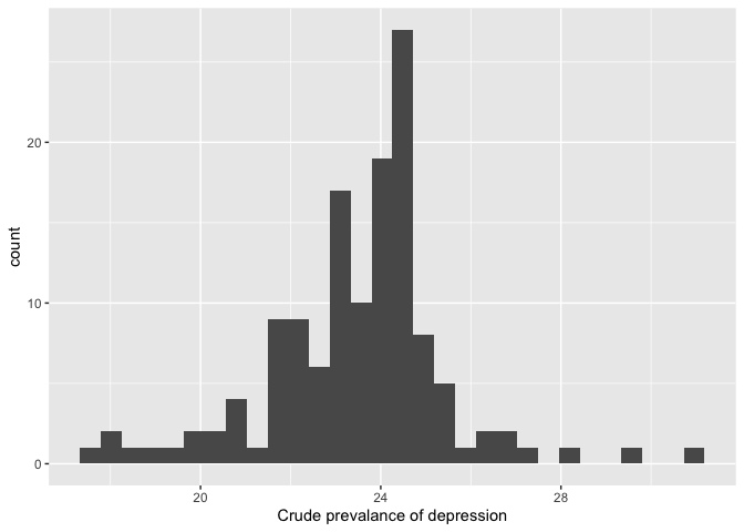

Run some of the other descriptive statistics and exploratory graphics covered in Lab 2 and check out Chapter 7 in RDS for more on EDA.

Standard linear regression

Our task is to examine the relationship between neighborhood socioeconomic and demographic characteristics and depression prevalence at the neighborhood level. Let’s first run a simple linear regression. The outcome is depression prevalence DEP_CrudePrev and the independent variable is poverty rate ppov (I start with the poverty rate for no special reason). We estimate regression models in R using the function lm(). We save the results of the model into the object fit.ols.simple.

fit.ols.simple <- lm(DEP_CrudePrev ~ ppov, data = sea.tracts)

The first argument in lm() takes on a formula object. A formula is indicated by a tilde ~. The dependent variable DEP_CrudePrev comes first, followed by the tilde ~, and then the independent variables. You can run generalized linear models, which allows you to run different types of regression models (e.g. logit) using the function glm().

We can look at a summary of results using the summary() function

summary(fit.ols.simple)

## 
## Call:
## lm(formula = DEP_CrudePrev ~ ppov, data = sea.tracts)
## 
## Residuals:
##     Min      1Q  Median      3Q     Max 
## -6.4303 -0.7182  0.4342  1.2641  4.8577 
## 
## Coefficients:
##             Estimate Std. Error t value Pr(>|t|)    
## (Intercept) 22.75899    0.25694  88.579  < 2e-16 ***
## ppov         0.06304    0.01700   3.708 0.000306 ***
## ---
## Signif. codes:  0 '***' 0.001 '**' 0.01 '*' 0.05 '.' 0.1 ' ' 1
## 
## Residual standard error: 1.912 on 132 degrees of freedom
## Multiple R-squared:  0.09434,    Adjusted R-squared:  0.08748 
## F-statistic: 13.75 on 1 and 132 DF,  p-value: 0.0003063

The output provides a lot of information. The most important are the coefficient estimates (under “Estimate”), standard errors (under “Std. Error”), and p-values (under “Pr(>|t|)”). The summary also provides model fit statistics at the bottom of the output (e.g. R-squared, F stat).

Practice Question: What does the value of the coefficient for ppov mean? Is the value statistically significant from 0? Based on what significance threshold(s)? What is the interpretation of the R² value?

Let’s next run a multiple linear regression. In addition to the poverty rate ppov, we will include the percent of residents who moved in the past year pmob, percent of 25 year olds with a college degree pcol, unemployment rate unempr, percent non-Hispanic black pnhblk, percent Hispanic phisp, and the log population size (I logged the size to make the coefficient a little easier to read). We save the results of the model into the object fit.ols.multiple.

fit.ols.multiple <- lm(DEP_CrudePrev ~ unempr + pmob + pcol + ppov + pnhblk + 
                phisp + log(tpop), data = sea.tracts)

The independent variables are separated by the + sign. Note that I logged population size using the function log(). We can look at a summary of results using the summary() function

summary(fit.ols.multiple)

## 
## Call:
## lm(formula = DEP_CrudePrev ~ unempr + pmob + pcol + ppov + pnhblk + 
##     phisp + log(tpop), data = sea.tracts)
## 
## Residuals:
##     Min      1Q  Median      3Q     Max 
## -5.2035 -0.7811  0.0631  1.0208  4.6762 
## 
## Coefficients:
##              Estimate Std. Error t value Pr(>|t|)    
## (Intercept) 15.908865   3.247366   4.899 2.90e-06 ***
## unempr      -0.007734   0.071401  -0.108 0.913918    
## pmob         0.005815   0.016979   0.342 0.732577    
## pcol         0.045214   0.014485   3.121 0.002233 ** 
## ppov         0.116605   0.023115   5.045 1.55e-06 ***
## pnhblk      -0.082835   0.022933  -3.612 0.000437 ***
## phisp        0.087031   0.034115   2.551 0.011936 *  
## log(tpop)    0.386229   0.387720   0.996 0.321085    
## ---
## Signif. codes:  0 '***' 0.001 '**' 0.01 '*' 0.05 '.' 0.1 ' ' 1
## 
## Residual standard error: 1.56 on 126 degrees of freedom
## Multiple R-squared:  0.4246, Adjusted R-squared:  0.3927 
## F-statistic: 13.28 on 7 and 126 DF,  p-value: 9.48e-13

A positive coefficient represents a positive association with depression status. We use a p-value threshold of 0.05 to indicate a significant result (e.g. a p-value less than 0.05 indicates that the coefficient is significantly different from 0 or no association). It appears that higher poverty rates, % college educated, and % Hispanic are associated with higher depression prevalence, whereas higher percent Black is associated with lower prevalence.

Diagnostics

R has some useful commands for running diagnostics to see if a regression model has some problems, specifically if it’s breaking any of the OLS assumptions outlined in Handout 7. One assumption is that the errors are normally distributed. We can visually inspect for violations of this assumption using a number of different charts and plots. First, we can create a basic histogram of the residuals. To extract the residuals from the saved regression model, use the function resid().

ggplot() + 
  geom_histogram(mapping = aes(x=resid(fit.ols.multiple))) +
  xlab("OLS residuals")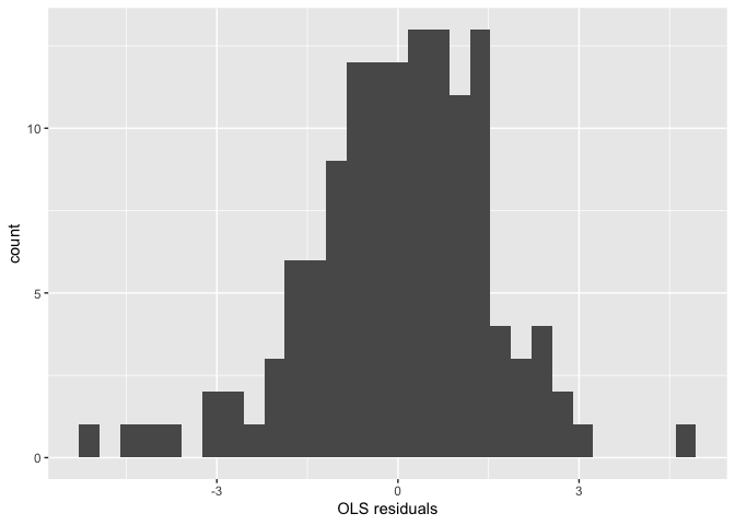

Normally distributed residuals should show a bell curve pattern. One problem with the histogram is its sensitivity to the choice of breakpoints for the bars - small changes can alter the visual impression quite drastically in some cases.

Another visual tool for checking normality is the quantile-quantile (Q-Q) plot, which plots the quantile of the residuals against the expected quantile of the standard normal distribution. We use the function qqPlot(), which is a part of the car package.

qqPlot(fit.ols.multiple)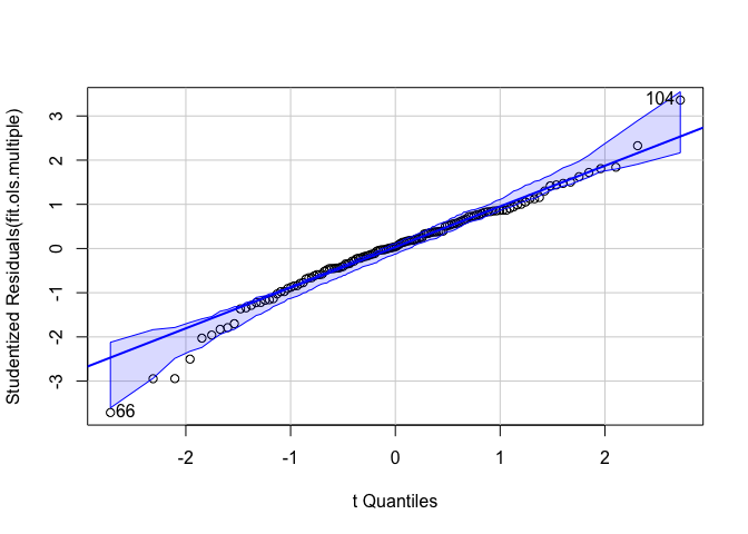

## [1]  66 104

The above figure is a quantile-comparison plot, graphing for each observation its fit.ols.multiple model residual on the y axis and the corresponding quantile in the t-distribution on the x axis. In contrast to the histogram, the q-q plot is more straightforward and effective and it is generally easier to assess whether the points are close to the diagonal line. The dashed lines indicate 95% confidence intervals calculated under the assumption that the errors are normally distributed. If a significant number of observations fall outside this range, this is an indication that the normality assumption has been violated. It looks like the vast majority of our points are within the band.

Another assumption is that errors are not heteroskedastic - that is the variance of residuals are constant. You can plot the residuals to explore the presence of heteroskedasticity. If we see the spread of the points narrow or widen from left to right, or we detect some kind of pattern rather than a cloud of points, heteroskedasticity is present.

plot(resid(fit.ols.multiple))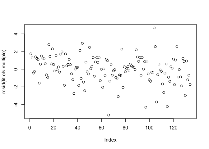

There appears to be no clear pattern, although there is a somewhat greater spread of points as you move left to right.

We won’t go through all the tools and approaches to testing the OLS assumptions (and other OLS issues) because it is beyond the scope of this course. In this lab, we’re interested in determining whether our models need to incorporate spatial dependency, an issue if not corrected will break assumptions 3 and 5 in Handout 7. We focus on this task in the following sections.

Exploratory Spatial Data Analysis

The above sections go through the steps conducted in non spatial regression analysis. The focus of this lab, however, is to account for spatial dependence in the error term and the dependent variable. Before doing any kind of spatial modelling, you should conduct an Exploratory Spatial Data Analysis (ESDA) to gain an understanding of how your data are spatially structured. ESDA is a subset of EDA methods that focus on the distinguishing characteristics of geographical data and, specifically, on spatial autocorrelation and spatial heterogeneity. ESDA techniques can help detect spatial patterns in data, lead to the formulation of hypotheses based on the geography of the data, and in assessing spatial models.

Map your data

The first step in ESDA is to map your dependent variable. Let’s map neighborhood depression prevalence using our trusty friend tm_shape(). You want to visually detect for spatial dependency or autocorrelation in your outcome.

tm_shape(sea.tracts, unit = "mi") +
  tm_polygons(col = "DEP_CrudePrev", style = "quantile",palette = "Reds", 
              border.alpha = 0, title = "") +
  tm_scale_bar(breaks = c(0, 2, 4), text.size = 1, position = c("right", "bottom")) +
  tm_layout(main.title = "Poor Mental Health Prevalence, Seattle 2017 ",  main.title.size = 0.95, frame = FALSE, legend.outside = TRUE, 
            attr.outside = TRUE)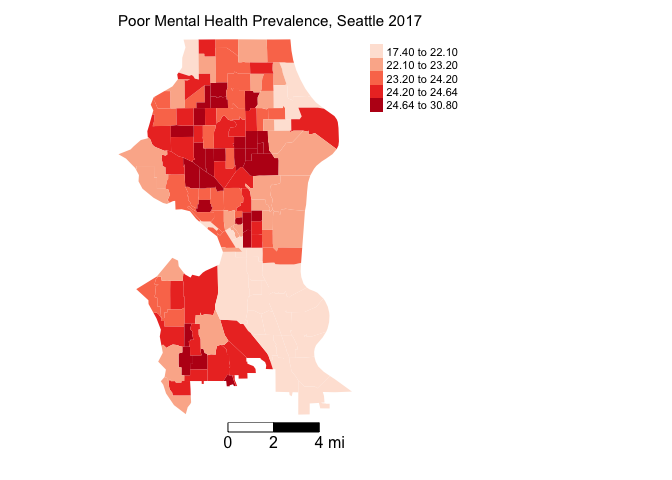

Next, you’ll want to map the residuals from your OLS regression model to see if there is visual evidence of spatial autocorrelation in the error. To extract the residuals from fit.ols.multiple, use the resid() function. Save it back into sea.tracts.

sea.tracts <- sea.tracts %>%
              mutate(olsresid = resid(fit.ols.multiple))

Plot the residuals.

tm_shape(sea.tracts, unit = "mi") +
  tm_polygons(col = "olsresid", style = "quantile",palette = "Reds", 
              border.alpha = 0, title = "") +
  tm_scale_bar(breaks = c(0, 2, 4), text.size = 1, position = c("right", "bottom")) +
  tm_layout(main.title = "Residuals from linear regression in Seattle Tracts",  main.title.size = 0.95, frame = FALSE, legend.outside = TRUE,
            attr.outside = TRUE)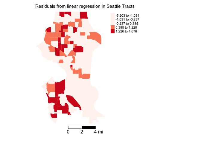

Both the outcome and the residuals appear to cluster.

Spatial Autocorrelation

There appears to be evidence of clustering based on the exploratory maps. Rather than eyeballing it, let’s formally test it by using a measure of spatial autocorrelation, which we covered in Lab 7. Before we do so, we need to create a spatial weights matrix, which we also covered in Lab 7. Let’s use Queen contiguity with row-standardized weights. First, create the neighbor nb object using poly2nb().

seab<-poly2nb(sea.tracts, queen=T)

Then the listw weights object using nb2listw().

seaw<-nb2listw(seab, style="W", zero.policy = TRUE)

Next, examine the Moran scatterplot, which we covered in Lab 7.

moran.plot(as.numeric(scale(sea.tracts$DEP_CrudePrev)), listw=seaw, 
           xlab="Standardized Depression Prevalence", 
           ylab="Neighbors Standardized Depression Prevalence",
           main=c("Moran Scatterplot for Depression Prevalence", "in Seatte") )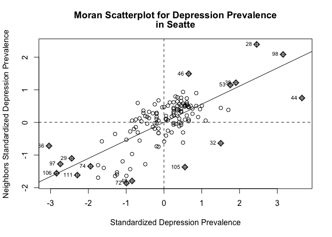

Does it look like there is an association? Yes.

Finally, the Global Moran’s I. We use Monte Carlo simulation to get the p-value.

moran.mc(sea.tracts$DEP_CrudePrev, seaw, nsim=999)

## 
##  Monte-Carlo simulation of Moran I
## 
## data:  sea.tracts$DEP_CrudePrev 
## weights: seaw  
## number of simulations + 1: 1000 
## 
## statistic = 0.55409, observed rank = 1000, p-value = 0.001
## alternative hypothesis: greater

Repeat for the OLS residuals using the lm.morantest() function.

lm.morantest(fit.ols.multiple, seaw)

## 
##  Global Moran I for regression residuals
## 
## data:  
## model: lm(formula = DEP_CrudePrev ~ unempr + pmob + pcol + ppov +
## pnhblk + phisp + log(tpop), data = sea.tracts)
## weights: seaw
## 
## Moran I statistic standard deviate = 6.6676, p-value = 1.3e-11
## alternative hypothesis: greater
## sample estimates:
## Observed Moran I      Expectation         Variance 
##      0.309531239     -0.026084108      0.002533614

Both the dependent variable and the residuals indicate spatial autocorrelation.

Practice Question: You should use other spatial weight matrices to test the robustness of your ESDA results. For example, do you get similar results using a 3-nearest neighbor definition? What about a 2000 meter definition?

Spatial lag model

Based on the exploratory mapping, Moran scatterplot, and the global Moran’s I, there appears to be spatial autocorrelation in the dependent variable. This means that if there is a spatial lag process going on and we fit an OLS model our coefficients will be biased and inefficient. That is, the coefficient sizes and signs are not close to their true value and its standard errors are underestimated. This means trouble. Big trouble. Real big trouble.

As outlined in Handout 7, there are two standard types of spatial regression models: a spatial lag model, which models dependency in the outcome, and a spatial error model, which models dependency in the residuals. A spatial lag model (SLM) can be estimated in R using the command lagsarlm(), which is a part of the spatialreg package.

fit.lag<-lagsarlm(DEP_CrudePrev ~ unempr + pmob+ pcol + ppov + pnhblk  + 
                    phisp + log(tpop),  
                  data = sea.tracts, 
                  listw = seaw)

The only real difference between the code for lm() and lagsarlm() is the argument listw, which you use to specify the spatial weights matrix. Get a summary of the results.

summary(fit.lag)

## 
## Call:lagsarlm(formula = DEP_CrudePrev ~ unempr + pmob + pcol + ppov + 
##     pnhblk + phisp + log(tpop), data = sea.tracts, listw = seaw)
## 
## Residuals:
##        Min         1Q     Median         3Q        Max 
## -4.8517717 -0.6798833 -0.0062064  0.8057965  3.4485538 
## 
## Type: lag 
## Coefficients: (asymptotic standard errors) 
##              Estimate Std. Error z value  Pr(>|z|)
## (Intercept)  5.727024   3.096952  1.8492 0.0644224
## unempr       0.010999   0.056872  0.1934 0.8466391
## pmob         0.012545   0.013697  0.9160 0.3596928
## pcol         0.021770   0.011922  1.8259 0.0678581
## ppov         0.071457   0.019183  3.7251 0.0001953
## pnhblk      -0.023195   0.018387 -1.2615 0.2071300
## phisp        0.048647   0.027398  1.7755 0.0758099
## log(tpop)    0.065312   0.309822  0.2108 0.8330399
## 
## Rho: 0.61792, LR test value: 40.638, p-value: 1.8322e-10
## Asymptotic standard error: 0.076375
##     z-value: 8.0906, p-value: 6.6613e-16
## Wald statistic: 65.457, p-value: 5.5511e-16
## 
## Log likelihood: -225.2712 for lag model
## ML residual variance (sigma squared): 1.5437, (sigma: 1.2425)
## Number of observations: 134 
## Number of parameters estimated: 10 
## AIC: 470.54, (AIC for lm: 509.18)
## LM test for residual autocorrelation
## test value: 0.049113, p-value: 0.82461

The summary output is very similar to the one produced by lm(). Only percent poverty is statistically significant. In the spatial lag model you will notice that there is a new term Rho. What is this? This is the spatial lag. It is a variable that measures depression prevalence in the tracts that are defined as surrounding each tract in the spatial weights matrix. We are using this variable as an additional explanatory variable to the model, so that we can appropriately take into account the spatial clustering detected by the Moran’s I test. You will notice that the estimated coefficient for this term is both positive and statistically significant (LR test, Z-test, and the Wald test). In other words, when depression prevalence in surrounding neighborhoods increases, on average, so does depression prevalence in each tract, even when we adjust for the other explanatory variables in the model. The fact the lag is significant adds further evidence that this is a better model than the OLS regression specification. There are some fit statistics located at the bottom of the summary, notably the AIC, and an LM test detecting whether spatial autocorrelation in the residuals still exist.

It may be tempting to compare the SLM and OLS regression coefficients. But you should be careful when doing this. Their meaning now has changed:

“Interpreting the substantive effects of each predictor in a spatial lag model is much more complex than in a nonspatial model (or in a spatial error model) because of the presence of the spatial multiplier that links the independent variables to the dependent. In the nonspatial model, it does not matter which unit is experiencing the change on the independent variable. The effect” in the dependent variable “of a change” in the value of an independent variable “is constant across all observations” (Darmofal, 2015: 107).

In the spatial lag model there are two components to how X affects Y. X affects Y within tract 1 directly. So our model includes the effect of X in tract 1 in the level of Y in tract 1. But remember we are also including the spatial lag, the measure of Y in the surrounding tracts (call them 2, 3, and 4). By virtue of including the spatial lag (a measure of Y in tracts 2, 3 and 4) we are indirectly incorporating as well the effect that X has on Y in tracts 1, 2, and 3. So the effect of a covariate (independent variable) is the sum of two particular effects: a direct, local effect of the covariate in that unit, and an indirect, spillover effect due to the spatial lag.

To get estimates of the direct, indirect and total effect of each variable, use the function impacts(). You need to include the lag model object, the spatial weights matrix, and the number of Monte Carlo simulations to obtain simulated distributions of the impacts (this used primarily for getting the standard errors for statistical inference).

fit.lag.effects <- impacts(fit.lag, listw = seaw, R = 999)
fit.lag.effects

## Impact measures (lag, exact):
##                Direct    Indirect       Total
## unempr     0.01220109  0.01658709  0.02878817
## pmob       0.01391597  0.01891843  0.03283439
## pcol       0.02414790  0.03282850  0.05697640
## ppov       0.07926360  0.10775697  0.18702056
## pnhblk    -0.02572841 -0.03497716 -0.06070558
## phisp      0.05396106  0.07335877  0.12731983
## log(tpop)  0.07244691  0.09848984  0.17093675

To get the standard errors, you use the summary() function and ask it to report the test statistic (Z) and the associated p-values.

summary(fit.lag.effects, zstats = TRUE, short = TRUE)

## Impact measures (lag, exact):
##                Direct    Indirect       Total
## unempr     0.01220109  0.01658709  0.02878817
## pmob       0.01391597  0.01891843  0.03283439
## pcol       0.02414790  0.03282850  0.05697640
## ppov       0.07926360  0.10775697  0.18702056
## pnhblk    -0.02572841 -0.03497716 -0.06070558
## phisp      0.05396106  0.07335877  0.12731983
## log(tpop)  0.07244691  0.09848984  0.17093675
## ========================================================
## Simulation results ( variance matrix):
## ========================================================
## Simulated standard errors
##               Direct   Indirect      Total
## unempr    0.06417668 0.10027582 0.16251547
## pmob      0.01490602 0.02363110 0.03776942
## pcol      0.01316602 0.01939196 0.03123798
## ppov      0.01979681 0.04341410 0.05626067
## pnhblk    0.01976839 0.03170915 0.05010837
## phisp     0.03111457 0.05164629 0.07936707
## log(tpop) 0.34777190 0.53383194 0.87116024
## 
## Simulated z-values:
##               Direct   Indirect      Total
## unempr     0.1780967  0.1589506  0.1684058
## pmob       0.9565514  0.8372409  0.9013455
## pcol       1.7795228  1.6486323  1.7734647
## ppov       3.9600272  2.5590824  3.3681816
## pnhblk    -1.2824744 -1.1364673 -1.2251220
## phisp      1.7247077  1.4551755  1.6230656
## log(tpop)  0.2247132  0.2179485  0.2232618
## 
## Simulated p-values:
##           Direct     Indirect Total     
## unempr    0.858647   0.873708 0.86626402
## pmob      0.338794   0.402457 0.36740464
## pcol      0.075154   0.099223 0.07615174
## ppov      7.4941e-05 0.010495 0.00075666
## pnhblk    0.199676   0.255761 0.22052926
## phisp     0.084580   0.145621 0.10457539
## log(tpop) 0.822202   0.827469 0.82333176

The impacts() function requires some matrix multiplication to generate these estimates. If you have a really large dataset (and hence a really large variance-covariance matrix), this will take a long time to run. If you either don’t have the time or the memory space, you can follow the approximation methods described in Lesage and Pace, 2009 that converts the spatial weight matrix into a “sparse” matrix”, and powers it up using the trW() function. It prepares a vector of traces of powers of a spatial weights matrix. The code for doing this is below, but I didn’t run it since our sample size is small enough to run impacts() quickly. The trW() function needs our spatial weights to be in a sparse matrix class object, so we can transform this using the as() function

#creates a sparse weights matrix
W <- as(seaw, "CsparseMatrix")
#creates a vector of traces of powers of the spatial weights matrix 
trMC <- trW(W, type="MC")
#direct, indirect and total effects
fit.lag.effects.sparse <- impacts(fit.lag, tr = trMC, R = 999)

Practice Question: In your own words, interpret the meaning of the direct, indirect and total effects of the variable ppov.

Spatial error model

The spatial error model (SEM) incorporates spatial dependence in the errors. If there is a spatial error process going on and we fit an OLS model our coefficients will be unbiased but inefficient. That is, the coefficient size and sign are asymptotically correct but its standard errors are underestimated.

We can estimate a spatial error model in R using the command errorsarlm() also in the spatialreg package.

fit.err<-errorsarlm(DEP_CrudePrev ~ unempr + pmob+ pcol + ppov + pnhblk  + 
                      phisp + log(tpop),  
                    data = sea.tracts, 
                    listw = seaw)

A summary of the modelling results

summary(fit.err)

## 
## Call:errorsarlm(formula = DEP_CrudePrev ~ unempr + pmob + pcol + ppov + 
##     pnhblk + phisp + log(tpop), data = sea.tracts, listw = seaw)
## 
## Residuals:
##      Min       1Q   Median       3Q      Max 
## -4.03421 -0.69122  0.18341  0.72580  3.47567 
## 
## Type: error 
## Coefficients: (asymptotic standard errors) 
##               Estimate Std. Error z value  Pr(>|z|)
## (Intercept) 24.3772615  2.5194147  9.6758 < 2.2e-16
## unempr       0.0194682  0.0482182  0.4038    0.6864
## pmob         0.0465997  0.0147655  3.1560    0.0016
## pcol         0.0100283  0.0144532  0.6938    0.4878
## ppov         0.0809183  0.0187238  4.3217 1.548e-05
## pnhblk       0.0062863  0.0202024  0.3112    0.7557
## phisp        0.0365228  0.0263092  1.3882    0.1651
## log(tpop)   -0.4395438  0.2791765 -1.5744    0.1154
## 
## Lambda: 0.80044, LR test value: 59.094, p-value: 1.4988e-14
## Asymptotic standard error: 0.055839
##     z-value: 14.335, p-value: < 2.22e-16
## Wald statistic: 205.49, p-value: < 2.22e-16
## 
## Log likelihood: -216.0433 for error model
## ML residual variance (sigma squared): 1.2327, (sigma: 1.1103)
## Number of observations: 134 
## Number of parameters estimated: 10 
## AIC: 452.09, (AIC for lm: 509.18)

The summary output is very similar to the one produced by the spatial lag model. The percent of residents who moved in the past year and percent poverty are positively associated with depression prevalence. Instead of Rho, the lag error parameter is Lambda, which is a lag on the error. It is positive and significant across all tests, indicating the need to control for spatial autocorrelation in the error.

Unlike the spatial lag, we don’t need to run impacts(), and thus the coefficients can be directly compared to the OLS coefficients.

Presenting your results

An organized table of results is an essential component not just in academic papers, but in any professional report or presentation. Up till this point, we’ve been reporting results by simply summarizing objects, like the following

summary(fit.ols.multiple)

We can make these results prettier by using a couple of functions for making nice tables in R. First, there is the as_flextable() function from the flextable package.

fit.ols.multiple %>% 
  as_flextable()

	Estimate	Standard Error	t value	Pr(>\|t\|)
(Intercept)	15.909	3.247	4.899	0.0000	***
unempr	-0.008	0.071	-0.108	0.9139
pmob	0.006	0.017	0.342	0.7326
pcol	0.045	0.014	3.121	0.0022	**
ppov	0.117	0.023	5.045	0.0000	***
pnhblk	-0.083	0.023	-3.612	0.0004	***
phisp	0.087	0.034	2.551	0.0119	*
log(tpop)	0.386	0.388	0.996	0.3211
Signif. codes: 0 <= '*' < 0.001 < '' < 0.01 < '*' < 0.05

Residual standard error: 1.56 on 126 degrees of freedom
Multiple R-squared: 0.4246, Adjusted R-squared: 0.3927
F-statistic: 13.28 on 126 and 7 DF, p-value: 0.0000

There are options within as_flextable() to control whether row names are included or not, column alignment, and other options that depend on the output type.

The table produced by as_flextable()looks good. But what if we want to present results for more than one model, such as presenting fit.ols.multiple, fit.lag, and fit.err side by side? We can use the stargazer() function from the stargazer package to do this.

stargazer(fit.ols.multiple, fit.lag, fit.err, type = "html",
                    title="Title: Regression Results")

**Title: Regression Results**

	Dependent variable:

	DEP_CrudePrev
	OLS	spatial	spatial
		autoregressive	error
	(1)	(2)	(3)

unempr	-0.008	0.011	0.019
	(0.071)	(0.057)	(0.048)

pmob	0.006	0.013	0.047^***
	(0.017)	(0.014)	(0.015)

pcol	0.045^***	0.022^*	0.010
	(0.014)	(0.012)	(0.014)

ppov	0.117^***	0.071^***	0.081^***
	(0.023)	(0.019)	(0.019)

pnhblk	-0.083^***	-0.023	0.006
	(0.023)	(0.018)	(0.020)

phisp	0.087^**	0.049^*	0.037
	(0.034)	(0.027)	(0.026)

log(tpop)	0.386	0.065	-0.440
	(0.388)	(0.310)	(0.279)

Constant	15.909^***	5.727^*	24.377^***
	(3.247)	(3.097)	(2.519)


Observations	134	134	134
R²	0.425
Adjusted R²	0.393
Log Likelihood		-225.271	-216.043
sigma²		1.544	1.233
Akaike Inf. Crit.		470.542	452.087
Residual Std. Error	1.560 (df = 126)
F Statistic	13.284^*** (df = 7; 126)
Wald Test (df = 1)		65.457^***	205.489^***
LR Test (df = 1)		40.638^***	59.094^***

Note:	p<0.1; p<0.05; p<0.01

There are a number of options you can tweak to make the table more presentation ready, such as adding footnotes and changing column and row labels.

Note a few things: First, if you ran the stargazer() function above directly in your R console, you’ll get output that won’t make sense. Knit the document and you’ll see your pretty table. Second, you will need to add results = 'asis' as an R Markdown chunk option (```{r results = 'asis'}).

Picking a model

Akaike Information Criterion

As we discussed in this week’s handout, there are many fit statistics and tests to determine which model - OLS, SLM or SEM - is most appropriate. One way of deciding which model is appropriate is to examine the fit statistic Akaike Information Criterion (AIC), which is a index of sorts to indicate how close the model is to reality. A lower value indicates a better fitting model.

You can extract the AIC from a model by using the function AIC(), which is a part of the pre-installed stats package. What is the AIC for the regular OLS model?

AIC(fit.ols.multiple)

## [1] 509.1802

What about the spatial lag and error models?

AIC(fit.lag)

## [1] 470.5424

AIC(fit.err)

## [1] 452.0866

Let’s extract the AICs, save them in a vector and then present them in a table using flextable().

#Save AIC values
AICs<-c(AIC(fit.ols.multiple),AIC(fit.lag), AIC(fit.err))
labels<-c("OLS", "SLM","SEM" )

flextable(data.frame(Models=labels, AIC=round(AICs, 2)))

Models	AIC
OLS	509.18
SLM	470.54
SEM	452.09

Lagrange Multiplier test

Another popular set of tests proposed by Anselin (1988) (also see Anselin et al. 1996) are the Lagrange Multiplier (LM) tests. The test compares the a model’s fit relative to the OLS model. A test showing statistical significance rejects the OLS.

To run the LM tests in R, plug in the saved OLS model fit.ols.multiple into the function lm.LMtests(), which is a part of the spatialreg package.

lm.LMtests(fit.ols.multiple, listw = seaw, test = "all",  zero.policy=TRUE)

## 
##  Lagrange multiplier diagnostics for spatial dependence
## 
## data:  
## model: lm(formula = DEP_CrudePrev ~ unempr + pmob + pcol + ppov +
## pnhblk + phisp + log(tpop), data = sea.tracts)
## weights: seaw
## 
## LMerr = 33.292, df = 1, p-value = 7.931e-09
## 
## 
##  Lagrange multiplier diagnostics for spatial dependence
## 
## data:  
## model: lm(formula = DEP_CrudePrev ~ unempr + pmob + pcol + ppov +
## pnhblk + phisp + log(tpop), data = sea.tracts)
## weights: seaw
## 
## LMlag = 42.279, df = 1, p-value = 7.914e-11
## 
## 
##  Lagrange multiplier diagnostics for spatial dependence
## 
## data:  
## model: lm(formula = DEP_CrudePrev ~ unempr + pmob + pcol + ppov +
## pnhblk + phisp + log(tpop), data = sea.tracts)
## weights: seaw
## 
## RLMerr = 0.14917, df = 1, p-value = 0.6993
## 
## 
##  Lagrange multiplier diagnostics for spatial dependence
## 
## data:  
## model: lm(formula = DEP_CrudePrev ~ unempr + pmob + pcol + ppov +
## pnhblk + phisp + log(tpop), data = sea.tracts)
## weights: seaw
## 
## RLMlag = 9.136, df = 1, p-value = 0.002506
## 
## 
##  Lagrange multiplier diagnostics for spatial dependence
## 
## data:  
## model: lm(formula = DEP_CrudePrev ~ unempr + pmob + pcol + ppov +
## pnhblk + phisp + log(tpop), data = sea.tracts)
## weights: seaw
## 
## SARMA = 42.428, df = 2, p-value = 6.122e-10

Practice Question: Which model is “best”? Why?

This work is licensed under a Creative Commons Attribution-NonCommercial 4.0 International License.

Website created and maintained by Noli Brazil