Lab 4b: Mapping Twitter Data
CRD 230 - Spatial Methods in Community Research
Professor Noli Brazil
Februuary 1, 2023
In this lab you will learn how to bring in, clean, analyze and map social media data accessed from Twitter in R. You will use the Twitter RESTful API v2 to access data about both twitter users and what they are tweeting about. The objectives of this guide are
- Learn how to bring in Twitter user and tweet data using Twitter’s API
- Learn how to conduct basic textual analysis on tweets
- Learn how to map Twitter user locations and geotagged tweets
Why examine Twitter data? Twitter is one of the most popular micro blogging sites in the world where thousands of people exchange their thoughts daily in the form of tweets. Although far from perfect, these data have become treasure troves of information, giving several chances for analyzing people’s reactions. Twitter data have been used to examine sentiments toward COVID-19, climate change, and major social issues and events such as the George Floyd protests, and the dissemination of misinformation. They have also been used to examine urban mobility patterns and identify geographic clusters of depression.
Installing and loading packages
You’ll need to install the following packages in R. You only need to do this once, so if you’ve already installed these packages, skip the code. Also, don’t put these install.packages() in your R Markdown document. Copy and paste the code in the R Console.
install.packages("rtweet")
install.packages("tidytext")
You’ll need to load the following packages. Unlike installing, you will always need to load packages whenever you start a new R session. You’ll also always need to use library() in your R Markdown file.
library(tidyverse)
library(sf)
library(leaflet)
library(tigris)
library(rtweet)
library(tidytext)
Read in census geography
We will be mapping tweet locations within the Los Angeles metropolitan area. As such, we’ll need to bring its boundaries into R using the function core_based_statistical_areas(), which we learned about in Lab 3.
cb <- core_based_statistical_areas(year = 2020, cb = TRUE)

#keep los angeles metro
la.metro <- filter(cb, grepl("Los Angeles", NAME))
Accessing the Twitter API
You can access the Twitter API a couple of ways. For all methods, you will need to have a Twitter account, so if you don’t already have one, sign up for one here.
You can access tweets via the API in the following ways.
User
If you just want to test the package, or are not using the API for a long period of time, use the default authentication auth_setup_default() that comes with rtweet.
auth_setup_default()Which will look up your account on your browser and create a token and save it as default. Here, you will need to authorize the embedded rstats2twitter app (approve the browser popup). After doing so, your token will be created and saved/stored (for future sessions) for you! It will use the current logged in account on the default browser to detect the credentials needed for rtweet and save them as “default”.
See here to learn more about authentication.
Apps and Bots
If you plan to make heavy usage of the package to collect a lot of information over a long period of time, I recommend setting up an App or Bot. What is the difference between the two? According to rtweet’s official descriptions
App authentication allows you to act as if you were a Twitter app. You can’t perform operations that a user can (like posting a tweet or reading a DM), but you get higher rate limits on data collection operations.
Bot authentication allows you to create a fully automated Twitter bot that performs actions on its own behalf rather than on behalf of a human.
To do this, you will need to sign up for a Twitter developer account and set up an App through this account. You don’t need to do this to proceed in the lab, but below are the general steps for doing so, with fuller details here and here.
Using your Twitter account, apply for a developer account here. On the developer account splash page, click on “Sign up”.
The next screen asks you to describe yourself. I chose “Academic researcher.” Select “No” under “Will you make Twitter content or derived…” Click on “Let’s do this”.
You will then need to add a valid phone number if you did not supply one when you signed up for Twitter. Once this is done, agree to the terms and conditions.
You will get an authentification code through your email. Submit that code in the next screen.
You set up an App by creating a project. Navigate to the developer portal. Click on “Create Project”.
You’ll need to name your project: the name is unimportant for our purposes, but if you’re using it for a project, name it something appropriate.
The next screen asks for the use case. I selected “Doing academic research.”
The next screen asks for a project description. You can just say you’re a graduate student taking a class.
You’ll need to name your app: similar to the project name, the app name is unimportant for our purposes, but needs to be unique across all twitter apps. I used “crd230” so that’s already taken.
After you’ve created your app, you’ll see a screen that gives you some important information regarding your API key, API secret key and Bearer token. You’ll only see this once, so make sure to record it in a secure location. Don’t worry if you forget to save this data: you can always regenerate new values by clicking the “regenerate” button on the “keys and tokens” page. If you regenerate the previous values will cease to work, so do not use it to get different credentials for an authentication already in use.
You will also need to write down or save the Access token and Access secret. To get these, you can navigate to your newly created app under the Project & Apps header on the left panel. Click on “Keys and tokens” The access token and secret are located at the bottom of the page.
You’ve now set up your Twitter API app! To use the App, you will need to use the function rtweet_app(). To use the bot, use the function rtweet_bot(). We won’t be using these functions in this lab, but for more details, check rtweets offficial authentication vignette.
Loading in Tweets
To send a request for tweets to Twitter’s API use the function search_tweets(). Let’s collect the 1,000 most recent tweets that contain the word “Biden”.
biden_tweets <- search_tweets(q="Biden", n = 1000,
                               include_rts = FALSE, lang = "en")
The argument q = specifies the words you want to search for in quotes. You can search for multiple words by using “AND” or “OR.” For example, to search for tweets with the words “biden” or “kamala”, use q = "biden OR kamala. To search for tweets that contain both “biden” and “kamala”, use q = "biden AND kamala".
The argument n = specifies the number of tweets you want to bring in. Twitter rate limits cap the number of search results returned to 18,000 every 15 minutes. To request more than that, simply set retryonratelimit = TRUE and rtweet will wait for rate limit resets for you. However, don’t go overboard. Bringing in, say, 50,000+ tweets may requires multiple hours if not days to complete.
The argument include_rts = FALSE excludes retweets. The argument lang = "en" collects tweets in the English language. Note that the Twitter REST API limits all searches to the past 6-9 days. You will not retrieve any earlier results. The results from this lab were downloaded on January 31, 2023.
Take a look at the data.
glimpse(biden_tweets)
Practice Question: Take a look at the data set. For each column, try and work out what kind of information it contains, and whether or not it could be useful for any analysis.
Let’s collect tweets containing the word “trump”.
trump_tweets <- search_tweets(q="Trump", n = 1000,
                              include_rts = FALSE, lang = "en")
Check the data.
glimpse(trump_tweets)The data set contains many variables. These variables include the user (handle and name) who sent the tweet, the tweet text itself, hashtags used in the tweet, how many times the tweet has been retweeted, and much much more. See here for the data dictionary.
You can also collect tweets from an individual account, such as BarackObama, using the function get_timelines(). Note that this is restricted to the most recent 3,200 tweets from a single account (even if you change the n = argument to something even higher, like 10,000).
barack_tweets <- get_timeline(user = "BarackObama", n = 1000, include_rts = FALSE)Take a look at the data
glimpse(barack_tweets)## Rows: 940
## Columns: 43
## $ created_at <dttm> 2023-01-28 10:15:25, 2023-01-28 10:15:0…
## $ id <dbl> 1.619399e+18, 1.619399e+18, 1.618982e+18…
## $ id_str <chr> "1619398759175319553", "1619398691621584…
## $ full_text <chr> "Along with mourning Tyre and supporting…
## $ truncated <lgl> FALSE, FALSE, FALSE, FALSE, FALSE, FALSE…
## $ display_text_range <dbl> 236, 225, 268, 195, 250, 238, 278, 255, …
## $ entities <list> [[<data.frame[1 x 2]>], [<data.frame[1 …
## $ source <chr> "<a href=\"http://twitter.com/download/i…
## $ in_reply_to_status_id <dbl> 1.619399e+18, NA, 1.618982e+18, NA, 1.61…
## $ in_reply_to_status_id_str <chr> "1619398691621584898", NA, "161898196511…
## $ in_reply_to_user_id <int> 813286, NA, 813286, NA, 813286, NA, 8132…
## $ in_reply_to_user_id_str <chr> "813286", NA, "813286", NA, "813286", NA…
## $ in_reply_to_screen_name <chr> "BarackObama", NA, "BarackObama", NA, "B…
## $ geo <list> NA, NA, NA, NA, NA, NA, NA, NA, NA, NA,…
## $ coordinates <list> [<data.frame[1 x 3]>], [<data.frame[1 x…
## $ place <list> [<data.frame[1 x 3]>], [<data.frame[1 x…
## $ contributors <lgl> NA, NA, NA, NA, NA, NA, NA, NA, NA, NA, …
## $ is_quote_status <lgl> FALSE, FALSE, FALSE, FALSE, FALSE, FALSE…
## $ retweet_count <int> 3225, 15371, 725, 2097, 391, 711, 1498, …
## $ favorite_count <int> 16367, 106079, 5443, 21391, 2374, 5366, …
## $ favorited <lgl> FALSE, FALSE, FALSE, FALSE, FALSE, FALSE…
## $ retweeted <lgl> FALSE, FALSE, FALSE, FALSE, FALSE, FALSE…
## $ possibly_sensitive <lgl> FALSE, FALSE, NA, NA, FALSE, FALSE, NA, …
## $ lang <chr> "en", "en", "en", "en", "en", "en", "en"…
## $ quoted_status_id <dbl> NA, NA, NA, NA, NA, NA, NA, NA, NA, 1.61…
## $ quoted_status_id_str <chr> NA, NA, NA, NA, NA, NA, NA, NA, NA, "161…
## $ quoted_status_permalink <list> [<data.frame[1 x 3]>], [<data.frame[1 x…
## $ quoted_status <list> [<data.frame[1 x 26]>], [<data.frame[1 …
## $ text <chr> "Along with mourning Tyre and supporting…
## $ favorited_by <lgl> NA, NA, NA, NA, NA, NA, NA, NA, NA, NA, …
## $ scopes <lgl> NA, NA, NA, NA, NA, NA, NA, NA, NA, NA, …
## $ display_text_width <lgl> NA, NA, NA, NA, NA, NA, NA, NA, NA, NA, …
## $ retweeted_status <lgl> NA, NA, NA, NA, NA, NA, NA, NA, NA, NA, …
## $ quote_count <lgl> NA, NA, NA, NA, NA, NA, NA, NA, NA, NA, …
## $ timestamp_ms <lgl> NA, NA, NA, NA, NA, NA, NA, NA, NA, NA, …
## $ reply_count <lgl> NA, NA, NA, NA, NA, NA, NA, NA, NA, NA, …
## $ filter_level <lgl> NA, NA, NA, NA, NA, NA, NA, NA, NA, NA, …
## $ metadata <lgl> NA, NA, NA, NA, NA, NA, NA, NA, NA, NA, …
## $ query <lgl> NA, NA, NA, NA, NA, NA, NA, NA, NA, NA, …
## $ withheld_scope <lgl> NA, NA, NA, NA, NA, NA, NA, NA, NA, NA, …
## $ withheld_copyright <lgl> NA, NA, NA, NA, NA, NA, NA, NA, NA, NA, …
## $ withheld_in_countries <lgl> NA, NA, NA, NA, NA, NA, NA, NA, NA, NA, …
## $ possibly_sensitive_appealable <lgl> NA, NA, NA, NA, NA, NA, NA, NA, NA, NA, …With get_timeline(), you are not limited to only the most recent 6-9 days of tweets.
Let’s also grab tweets from Bernie Sanders whose Twitter handle is BernieSanders
bernie_tweets <- get_timeline(user = "BernieSanders", n = 1000, include_rts = FALSE)Visualizing Tweets
rtweet includes the ts_plot() function which automates some common time series visualization methods. For example, we can quickly visualize the frequency of Bernie Sanders tweets.
ts_plot(bernie_tweets, by = "1 month")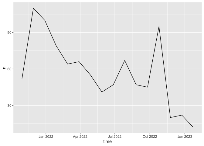
The by argument allows us to aggregate over different lengths of time.
Compared to President Obama?
ts_plot(barack_tweets, by = "1 month")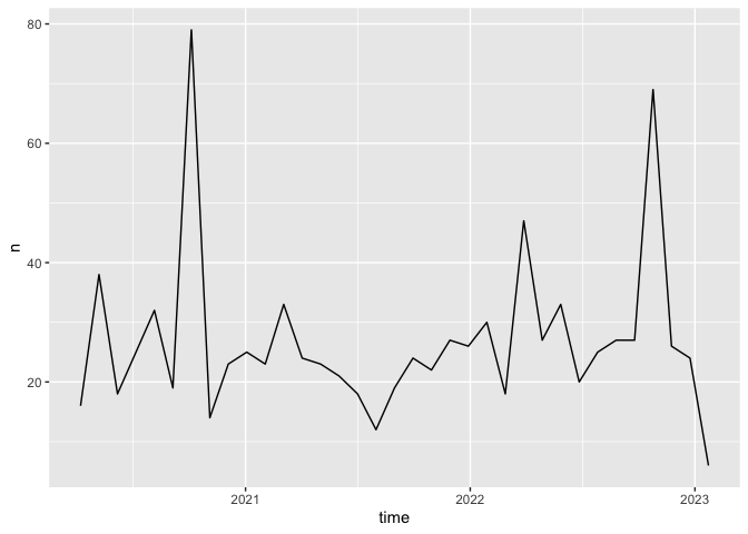
Practice Exercise: Can you think of a popular topic that might show temporal patterns (i.e.an increase or decrease over time)? Try it out! Collect some data using either search_tweets() or get_timelines(), then use ts_plot() to plot the frequency over time
Textual Analysis
Now that we’ve run through various ways of collecting tweets, let’s run over some basic text analysis you can conduct.
We can look at the content of these tweets in more detail by calculating the most frequent words.
First off, let’s convert our database of Bernie tweets so that each word of each tweet is on its own line. We can use unnest_tokens() which is part of the tidytext package to transform our dataframe into a one-word-per-line format.
bernie_words <- bernie_tweets %>%
  select(id, text) %>%
  unnest_tokens(word, text)
Let’s use head() to look at the first 6 lines, just to make sure our code has worked:
head(bernie_words)## # A tibble: 6 × 2
## id word
## <dbl> <chr>
## 1 1.62e18 there
## 2 1.62e18 is
## 3 1.62e18 nowhere
## 4 1.62e18 in
## 5 1.62e18 this
## 6 1.62e18 countryLooks good! Each line of bernie_words contains a single word from each tweet, with a column corresponding to the tweet ID containing that word. Now we’ve got each word of each tweet on its own line, we can simply count the occurrence of each word and plot the most frequent ones.
bernie_count <- bernie_words %>%
  count(word, sort = TRUE) %>%
  head(30) %>%
  mutate(word = reorder(word, n))
Now we can plot the word frequency using our best bud ggplot()
bernie_count %>%
  ggplot(aes(x = word, y = n)) +
  geom_col() +
  coord_flip() +
  theme_minimal()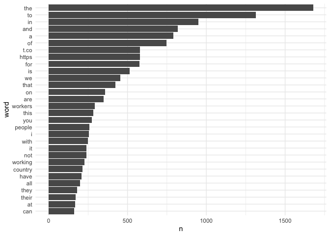
Cool! But there’s a problem here: obviously the most frequent words are things like the, to, and, of etc. which aren’t particularly interesting. To remove this, we can use what’s called a “stop list”, which is a list of highly frequent words you want to exclude from the analysis. Luckily, the tidytext package provides one of these, called stop_words. The following code adds a few Twitter-specific items to this list, such as hyperlinks (‘https’) and acronyms (‘rt’, i.e. ‘retweet’) that we obviously aren’t interested in.
new_items <- c("https", "t.co", "amp", "rt")

stop_words_new <- stop_words %>%
  pull(word) %>%
  append(new_items)
Now we can remake the bernie_count object, but with the addition of a new line that excludes certain words from our dataset
bernie_count <- bernie_words %>%
  filter(!word %in% stop_words_new) %>%
  count(word, sort = TRUE) %>%
  head(30) %>%
  mutate(word = reorder(word, n))
Then plot
bernie_count %>%
  ggplot(aes(x = word, y = n)) +
  geom_col() +
  coord_flip() +
  theme_minimal()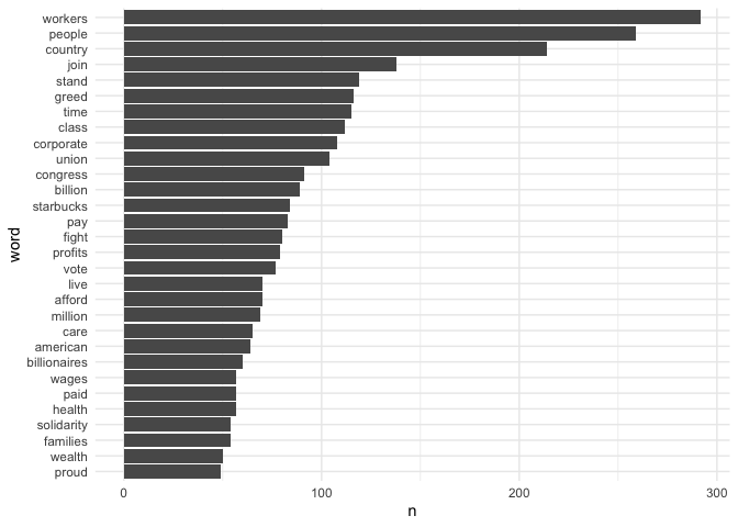
Sanders tweets a lot about ‘workers’, ‘people’ ‘join’, ‘greed’ and ‘class’.
n-grams
So far we’ve just looked at the frequency of individual words, but of course in language context is very important. For this reason, it’s quite common to investigate frequent collocations of words instead - or n-grams. Let’s test it out by looking at bigrams from Bernie’s tweets - i.e. which two words appear together most often?
We can use the unnest_tokens() like we did before to get a one-word-per-line format, but this time we include the token = "ngrams" and n = 2 arguments, which tells R to tokenise into bigrams instead of individual words (if we wanted trigrams, we would change n to 3)
bernie_ngrams <- bernie_tweets %>%
  select(id, text) %>%
  unnest_tokens(output = bigram, input = text, token = "ngrams", n = 2)
Take a look at the first 10 rows to make sure it’s worked:
head(bernie_ngrams)## # A tibble: 6 × 2
## id bigram
## <dbl> <chr>
## 1 1.62e18 there is
## 2 1.62e18 is nowhere
## 3 1.62e18 nowhere in
## 4 1.62e18 in this
## 5 1.62e18 this country
## 6 1.62e18 country whereCoolio. Next up, we need to count the number of occurrences of each bigram. We can do this using count(), as we did for individual lexical frequency earlier, but before we do that we should separate() each bigram into its constituent words and get rid of any that are in our stop list (stop_words_new) - we can do this using filter().
bernie_ngrams_count <- bernie_ngrams %>%
  separate(bigram, c("word1", "word2"), sep = " ") %>%
  filter(!word1 %in% stop_words_new & !word2 %in% stop_words_new) %>%
  count(word1, word2, sort = TRUE)
Now let’s plot them!
bernie_ngrams_count %>%
  mutate(bigram = paste(word1, word2)) %>%
  mutate(bigram = reorder(bigram, n)) %>%
  head(10) %>%
  ggplot(aes(x = bigram, y = n)) +
  geom_col() +
  coord_flip()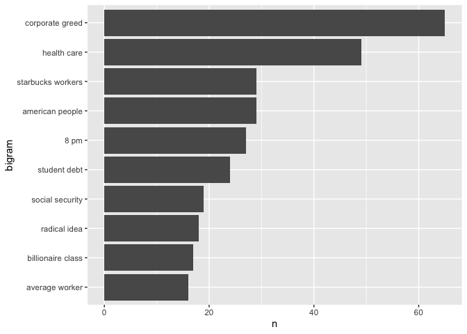
Do these n-grams align with Sanders political platform?
The text analysis we conducted above is just a small part of a broader set of tools known as sentiment analysis. Sentiment analysis is the process of computationally identifying and categorizing opinions expressed in a piece of text, especially in order to determine whether the writer’s attitude towards a particular topic, product, etc. is positive, negative, or neutral. Such an analysis is beyond the scope of the course, but if you’re interested, here is a good resource, and here is a recently published paper focusing on sentiment analysis of Twitter data.
Guess what? Badge time!

Visualizing Tweet Locations
In this lab we’re primarily interested in determining the geographic locations of tweets. To do so, we need to use search_tweets() again, but specify that you want tweets with geographic coordinates within the United States. First Trump (we’ll grab 8,000 of his most recent tweets containing the word “trump” AND have geographic coordinates within the United States - I bumped it up to 8,000 because it is considerably less likely to have tweets with geographic coordinates attached since providing the tweet location is voluntary).
trump_tweets_us <- search_tweets(q="Trump", n = 8000,
                              include_rts = FALSE, lang = "en",
                              geocode = lookup_coords("usa"))
Next Biden.
biden_tweets_us <- search_tweets(q="Biden", n = 8000,
                               include_rts = FALSE, lang = "en",
                             geocode = lookup_coords("usa"))
The argument geocode = lookup_coords("usa") collects tweets sent from the United States.
There are a couple of sources of geographic information in the data. First, you have geographic information embedded within the tweet itself. You can use search_tweets() to find all tweets that refer to a specific place (e.g. a city such as “los angeles” or a neighborhood such as Sacramento’s “oak park”).
Second, the user sets a place with a name such as “Los Angeles” in their tweet. In other words, the user tweets something and adds a place to where this tweet is being tweeted from. The variable containing the tweet place is place.
The third source for geographic information is the geotagged precise location point coordinates of where the tweet was tweeted. To extract the longitudes and latitudes of the tweet locations use the function lat_lng(). Let’s get the coordinates for the biden tweets.
biden_tweets_us <- lat_lng(biden_tweets_us)

#take a look at the data
glimpse(biden_tweets_us)
## Rows: 10
## Columns: 48
## $ created_at <dttm> 2023-01-31 20:43:09, 2023-01-31 20:38:2…
## $ id <dbl> 1.620644e+18, 1.620643e+18, 1.620643e+18…
## $ id_str <chr> "1620643895821598721", "1620642690961666…
## $ full_text <chr> "@RNCResearch We all realize Biden's men…
## $ truncated <lgl> FALSE, FALSE, FALSE, FALSE, FALSE, FALSE…
## $ display_text_range <dbl> 101, 89, 179, 113, 68, 197, 218, 283, 30…
## $ entities <list> [[<data.frame[1 x 2]>], [<data.frame[1 …
## $ metadata <list> [<data.frame[1 x 2]>], [<data.frame[1 x…
## $ source <chr> "<a href=\"http://twitter.com/download/a…
## $ in_reply_to_status_id <dbl> 1.620494e+18, NA, NA, NA, 1.620387e+18, …
## $ in_reply_to_status_id_str <chr> "1620494321760849921", NA, NA, NA, "1620…
## $ in_reply_to_user_id <dbl> 5.532916e+07, NA, NA, NA, 3.419211e+09, …
## $ in_reply_to_user_id_str <chr> "55329156", NA, NA, NA, "3419210573", "8…
## $ in_reply_to_screen_name <chr> "RNCResearch", NA, NA, NA, "FemalesForTr…
## $ geo <list> NA, NA, NA, NA, NA, NA, NA, NA, NA, NA
## $ coordinates <list> [<data.frame[1 x 3]>], [<data.frame[1 x…
## $ place <list> [<data.frame[1 x 3]>], [<data.frame[1 x…
## $ contributors <lgl> NA, NA, NA, NA, NA, NA, NA, NA, NA, NA
## $ is_quote_status <lgl> FALSE, FALSE, FALSE, FALSE, FALSE, FALS…
## $ retweet_count <int> 0, 0, 0, 0, 0, 0, 0, 0, 0, 1
## $ favorite_count <int> 0, 0, 0, 0, 0, 0, 0, 0, 0, 1
## $ favorited <lgl> FALSE, FALSE, FALSE, FALSE, FALSE, FALSE…
## $ retweeted <lgl> FALSE, FALSE, FALSE, FALSE, FALSE, FALSE…
## $ lang <chr> "en", "en", "en", "en", "en", "en", "en"…
## $ possibly_sensitive <list> NA, NA, FALSE, FALSE, FALSE, NA, NA, NA,…
## $ quoted_status <list> NA, NA, NA, NA, NA, NA, NA, NA, NA, NA
## $ text <chr> "@RNCResearch We all realize Biden's men…
## $ favorited_by <lgl> NA, NA, NA, NA, NA, NA, NA, NA, NA, NA
## $ scopes <lgl> NA, NA, NA, NA, NA, NA, NA, NA, NA, NA
## $ display_text_width <lgl> NA, NA, NA, NA, NA, NA, NA, NA, NA, NA
## $ retweeted_status <lgl> NA, NA, NA, NA, NA, NA, NA, NA, NA, NA
## $ quoted_status_id <lgl> NA, NA, NA, NA, NA, NA, NA, NA, NA, NA
## $ quoted_status_id_str <lgl> NA, NA, NA, NA, NA, NA, NA, NA, NA, NA
## $ quoted_status_permalink <lgl> NA, NA, NA, NA, NA, NA, NA, NA, NA, NA
## $ quote_count <lgl> NA, NA, NA, NA, NA, NA, NA, NA, NA, NA
## $ timestamp_ms <lgl> NA, NA, NA, NA, NA, NA, NA, NA, NA, NA
## $ reply_count <lgl> NA, NA, NA, NA, NA, NA, NA, NA, NA, NA
## $ filter_level <lgl> NA, NA, NA, NA, NA, NA, NA, NA, NA, NA
## $ query <lgl> NA, NA, NA, NA, NA, NA, NA, NA, NA, NA
## $ withheld_scope <lgl> NA, NA, NA, NA, NA, NA, NA, NA, NA, NA
## $ withheld_copyright <lgl> NA, NA, NA, NA, NA, NA, NA, NA, NA, NA
## $ withheld_in_countries <lgl> NA, NA, NA, NA, NA, NA, NA, NA, NA, NA
## $ possibly_sensitive_appealable <lgl> NA, NA, NA, NA, NA, NA, NA, NA, NA, NA
## $ lat <dbl> 41.50075, 31.99430, 44.31850, 42.49582, …
## $ lng <dbl> -72.75738, -102.10463, -89.90882, -82.89…
## $ coords_coords <I<list>> NA, NA, NA, NA, NA, NA, NA, NA, NA, NA,…
## $ bbox_coords <I<list>> -72.7573...., -102.104...., -89.9088...…
## $ geo_coords <I<list>> NA, NA, NA, NA, NA, NA, NA, NA, NA, NA, …The function creates two new columns in the data set, lat and lng, which represent the latitude and longitude coordinates, respectively.
Next, Trumpster
trump_tweets_us <- lat_lng(trump_tweets_us)An important issue to note is that Twitter requires users to decide whether they want to opt into allowing the company to collect geotagged information on their tweets. As a result of the change, it is estimated that 1-2% of tweets have geographic coordinate information.
Mapping Tweets
Now that we have the longitudes and latitudes of the tweets, we can map them. To do so, let’s follow Lab 4a and convert the non-spatial data frames biden_tweets_us and trump_tweets_us into sf objects using the st_as_sf() command.
biden_tweets.geo.sf <- st_as_sf(biden_tweets_us, coords = c("lng", "lat"), crs = "+proj=longlat +datum=WGS84 +ellps=WGS84")

trump_tweets.geo.sf <- st_as_sf(trump_tweets_us, coords = c("lng", "lat"), crs = "+proj=longlat +datum=WGS84 +ellps=WGS84")
Let’s use leaflet() to map the points. You can also use tm_shape() from the tmap package, which we learned about in Lab 3. First, let’s map the Biden tweets.
leaflet() %>%
  addProviderTiles("OpenStreetMap.Mapnik") %>%
  addCircles(data = biden_tweets.geo.sf,
             color = "blue")
Next, let’s map the Trumpy tweets.
leaflet() %>%
  addProviderTiles("OpenStreetMap.Mapnik") %>%
  addCircles(data = trump_tweets.geo.sf,
             color = "red")
Rather than the entire United States, let’s map tweets located within the Los Angeles Metropolitan Area. To do this, we’ll need to make sure the the sf object la.metro has the same CRS as biden_tweets.geo.sf.
st_crs(la.metro) == st_crs(biden_tweets.geo.sf)## [1] FALSELet’s reproject la.metro into the same CRS as biden_tweets.geo.sf using the function st_transform(), which we learned about in Lab 4a.
la.metro <-st_transform(la.metro, crs = st_crs(biden_tweets.geo.sf)) Let’s keep the Biden and Trump tweets within the metro area using the st_within option in the st_join() command, which we learned about in Lab 3.
biden_tweets.geo.la <- st_join(biden_tweets.geo.sf, la.metro, join = st_within, left=FALSE)
trump_tweets.geo.la <- st_join(trump_tweets.geo.sf, la.metro, join = st_within, left=FALSE)
Finally, use leaflet() to map the tweets on top of the metro area boundary.
leaflet() %>%
  addProviderTiles("OpenStreetMap.Mapnik") %>%
  addPolygons(data = la.metro,
              color = "gray",
              weight = 1,
              smoothFactor = 0.5,
              opacity = 1.0,
              fillOpacity = 0.2) %>%
  addCircles(data = biden_tweets.geo.la,
             color = "blue") %>%
  addCircles(data = trump_tweets.geo.la,
             color = "red")
You might be thinking that you can directly get tweets in Los Angeles using geocode = lookup_coords("los angeles, CA") in search_tweets(). You can but only if you have a Google Maps API Key, which requires you to provide a credit card number (to pay in case you go over their free limit). rtweet only allows you to narrow the tweets to the United States without a Google Maps API Key.
Mapping Twitter User Locations
The fourth source for Twitter geographic information is the location specified by the user in their account profile. This information is stored in the variable location. This variable (and other variables related to the user) can be extracted using the function users_data(). Let’s plot the top 10 locations of ALL users who tweeted “biden” (eliminating NA and blank values).
biden_tweets %>%
  users_data() %>%
  count(location, sort = TRUE) %>%
  mutate(location = reorder(location,n)) %>%
  filter(is.na(location) == FALSE & location != "") %>%
  top_n(10) %>%
  ggplot(aes(x = location,y = n)) +
  geom_col() +
  coord_flip() +
  labs(x = "Place",
       y = "Count",
       title = "Biden Tweet users - unique locations ")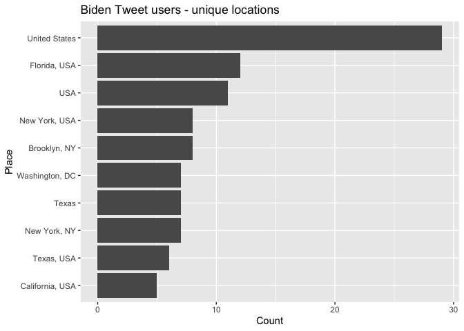
And Trumpy
trump_tweets %>%
  users_data() %>%
  count(location, sort = TRUE) %>%
  mutate(location = reorder(location,n)) %>%
  filter(is.na(location) == FALSE & location != "") %>%
  top_n(10) %>%
  ggplot(aes(x = location,y = n)) +
  geom_col() +
  coord_flip() +
  labs(x = "Place",
       y = "Count",
       title = "Trump Tweet users - unique locations ")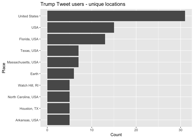
You can also search for users (not tweets) using the function search_users(). Twitter will look for matches in user names, screen names, and profile bios. Let’s look for users with the words “maga” somewhere in their profile bios, user names or screen names. The maximum number of users a single call returns is 1,000.
# what users are tweeting with MAGA
users <- search_users("MAGA",
                      n = 1000)
and the top 20 locations (eliminating NA and blank values)
users %>%
  count(location, sort = TRUE) %>%
  mutate(location = reorder(location,n)) %>%
  filter(is.na(location) == FALSE & location != "") %>%
  top_n(20) %>%
  ggplot(aes(x = location,y = n)) +
  geom_col() +
  coord_flip() +
  labs(x = "Location",
       y = "Count",
       title = "MAGA users - unique locations ")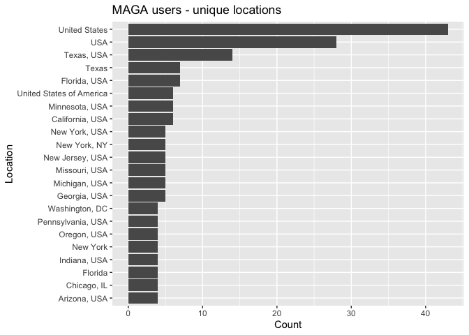
You can repeat the process of getting Longitude and Latitude coordinates of “MAGA” users and map them across the United States and within the Los Angeles Metropolitan Area.
You’ve completed the lab guide on how to use the package rtweet to bring in Twitter data. Hey, you know what? You earned a badge! Woohoo!


This work is licensed under a Creative Commons Attribution-NonCommercial 4.0 International License.
Website created and maintained by Noli Brazil